


🚀 Vectorized Logistic Regression in Python: From Scratch with NumPy
DL (Part 17)

📚Chapter 3 Python and Vectorization
If you want to read more articles about Deep Learning, don’t forget to stay tuned :) click here.
Description
In the previous tutorial, you saw how you can use vectorization to compute their predictions. The lowercase a’s for an entire training set all at the same time. In this Tutorial, you see how you can use vectorization to also perform the gradient computations for all M training samples. Again, all sort of at the same time. And then at the end of this Tutorial, we’ll put it all together and show how you can derive a very efficient implementation of logistic regression.
Sections
Vectorizing Logistic Regression
Implementing logistic Regression
Section 1: Why Vectorization Matters in Logistic Regression
Vectorization in machine learning isn't just a performance booster — it's a necessity for scaling your models efficiently. When you're working with large datasets, removing for-loops from your code can speed things up dramatically.
In this post, we’ll walk through how to:
Vectorize logistic regression forward and backward passes
Compute gradients efficiently
Implement a loop-free version of logistic regression in NumPy
Understand what's happening under the hood — without black-box magic
Let’s dive into how vectorization transforms basic logistic regression into a faster, cleaner implementation.

So, you may remember that for the gradient computation, what we did was we computed dz1 for the first example, which could be a1 minus y1 and then dz2 equals a2 minus y2 and so on. And so on for all M training examples. So, what we’re going to do is define a new variable, dZ is going to be dz1, dz2, dzm. Again, all the D lowercase z variables stacked horizontally. So, this would be 1 by m matrix or alternatively a m dimensional row vector. Now recall that from the previous slide, we’d already figured out how to compute capital A which was this: a1 through am and we had defined capital Y as y1 through ym. Also you know, stacked horizontally. So, based on these definitions, maybe you can see for yourself that dz can be computed as just A minus Y because it’s going to be equal to a1 — y1. So, the first element, a2 — y2, so in the second element and so on. And, so this first element a1 — y1 is exactly the definition of dz1. The second element is exactly the definition of dz2 and so on. So, with just one line of code, you can compute all of this at the same time. Now, in the previous implementation, we’ve gotten rid of one for loop already but we still had this second for loop over training examples. So we initialize dw to zero to a vector of zeroes. But then we still have to loop over 20 examples where we have dw plus equals x1 times dz1, for the first training example dw plus equals x2 dz2 and so on. So we do the M times and then dw divide equals by M and similarly for B, right? db was initialized as 0 and db plus equals dz1. db plus equals dz2 down to you know dz(m) and db divide equals M. So that’s what we had in the previous implementation. We’d already got rid of one for loop. So, at least now dw is a vector and we went separately updating dw1, dw2 and so on. So, we got rid of that already but we still had the for loop over the M examples in the training set. So, let’s take these operations and vectorize them. Here’s what we can do, for the vectorized implementation of db, what it’s doing is basically summing up, all of these dzs and then dividing by m. So, db is basically one over m, sum from I equals one through m of dzi and well all the dzs are in that row vector and so in Python, what you do is implement you know, 1 over a m times np. sum of dz. So, you just take this variable and call the np. sum function on it and that would give you db. How about dw? I’ll just write out the correct equations who can verify is the right thing to do. DW turns out to be one over M, times the matrix X times dz transpose. And, so kind of see why that’s the case. This is equal to one over m then the matrix X’s, x1 through xm stacked up in columns like that and dz transpose is going to be dz1 down to dz(m) like so. And so, if you figure out what this matrix times this vector works out to be, it is turns out to be one over m times x1 dz1 plus… plus xm dzm. And so, this is a n/1 vector and this is what you actually end up with, with dw because dw was taking these you know, xi dzi and adding them up and so that’s what exactly this matrix vector multiplication is doing and so again, with one line of code you can compute dw. So, the vectorized implementation of the derivative calculations is just this, you use this line to implement db and use this line to implement dw and notice that without a for loop over the training set, you can now compute the updates you want to your parameters.
Section 2- 🔄 What We’re Vectorizing: Forward and Backward Passes
In logistic regression, you predict outputs for M training examples using weights w and a bias b. Traditionally, you'd loop through each example to calculate predictions and update weights. But that’s slow.
With NumPy, we can replace these loops with matrix operations. Here's what we're optimizing:
Forward pass: Compute predictions
a = sigmoid(w.T @ X + b)Backward pass: Compute gradients
dwanddbefficientlyParameter updates: Adjust
wandbusing gradient descent — without using a loop per training sample
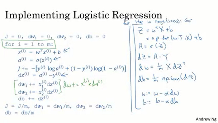
So now, let’s put all together into how you would actually implement logistic regression. So, this is our original, highly inefficient non vectorize implementation. So, the first thing we’ve done in the previous video was get rid of this volume, right? So, instead of looping over dw1, dw2 and so on, we have replaced this with a vector value dw which is dw+= xi, which is now a vector times dz(i). But now, we will see that we can also get rid of not just a for loop below but also get rid of this for loop. So, here is how you do it. So, using what we have from the previous slides, you would say, capitalZ, Z equal to w transpose X + B and the code you is write capital Z equals np. w transpose X + B and then a equals sigmoid of capital Z. So, you have now computed all of this and all of this for all the values of I. Next on the previous slide, we said you would compute dz equals A — Y. So, now you computed all of this for all the values of i. Then, finally dw equals 1/m x dz transpose and db equals 1/m of you know, np. sum dz. So, you’ve just done forward propagation and back propagation, really computing the predictions and computing the derivatives on all M training examples without using a for loop. And so the gradient descent update then would be you know W gets updated as w minus the learning rate times dw which was just computed above and B is update as B minus the learning rate times db. Sometimes is putting colons to that to denote that as is an assignment, but I guess I haven’t been totally consistent with that notation. But with this, you have just implemented a single iteration of gradient descent for logistic regression. Now, I know I said that we should get rid of explicit for loops whenever you can but if you want to implement multiple iterations as a gradient descent then you still need a for loop over the number of iterations. So, if you want to have a thousand iterations of gradient descent, you might still need a for loop over the iteration number. There is an outermost for loop like that then I don’t think there is any way to get rid of that for loop. But I do think it’s incredibly cool that you can implement at least one iteration of gradient descent without needing to use a for loop. So, that’s it you now have a highly vectorize and highly efficient implementation of gradient descent for logistic regression. There is just one more detail that I want to talk about in the next Tutorial, which is in our description here I briefly alluded to this technique called broadcasting. Broadcasting turns out to be a technique that Python and numpy allows you to use to make certain parts of your code also much more efficient. So, let’s see some more details of broadcasting in the next tutorial.
✍️ Vectorizing the Gradient Calculation
Let’s look at the backward pass, where we compute the gradient of the loss.
Assume:
Ais the prediction for all M samplesYis the true labelsXis your input matrix of shape (n_features, m_samples)
Step-by-step Gradient Computation
dZ = A - Y  # Vectorized error term
dw = (1/m) * X @ dZ.T  # Gradient w.r.t. weights
db = (1/m) * np.sum(dZ)  # Gradient w.r.t. bias
This replaces your manual loop where you used to update dw and db one example at a time. NumPy handles it all in one shot.
🧪 Full Python Example: Logistic Regression with Vectorization
Let’s see it all in action using a built-in dataset from sklearn.
Let’s see it all in action using a built-in dataset from sklearn.
import numpy as np
from sklearn.datasets import load_breast_cancer
from sklearn.model_selection import train_test_split
from sklearn.preprocessing import StandardScaler

# Load a simple binary classification dataset
data = load_breast_cancer()
X, y = data.data.T, data.target.reshape(1, -1)  # Transpose for consistency
m = X.shape[1]

# Standardize features
scaler = StandardScaler()
X = scaler.fit_transform(X.T).T  # Standardize and transpose back

# Initialize parameters
n_features = X.shape[0]
w = np.zeros((n_features, 1))
b = 0
learning_rate = 0.01
num_iterations = 1000

# Sigmoid function
def sigmoid(z):
    return 1 / (1 + np.exp(-z))

# Gradient descent
for i in range(num_iterations):
    Z = np.dot(w.T, X) + b            # Linear activation
    A = sigmoid(Z)                    # Sigmoid output
    dZ = A - y                        # Error term
    dw = (1/m) * np.dot(X, dZ.T)      # Gradient of weights
    db = (1/m) * np.sum(dZ)           # Gradient of bias

    # Update parameters
    w -= learning_rate * dw
    b -= learning_rate * db

# Prediction on training set
preds = sigmoid(np.dot(w.T, X) + b) > 0.5
accuracy = np.mean(preds == y)
print(f"Training accuracy: {accuracy * 100:.2f}%")
👨🏫 What Just Happened?
We used the Breast Cancer dataset from
sklearnVectorized forward and backward pass — no loops over examples
Used gradient descent to update the model
Achieved high accuracy — with clear, efficient code
🧠 Why This Matters
Efficient computation is a cornerstone of deep learning. Vectorizing your models helps:
Speed up training time
Keep code cleaner and easier to debug
Scale to larger datasets
This is the exact logic that powers deeper models — even in popular frameworks like TensorFlow and PyTorch.
🎯 Call to Action
Liked this tutorial?
👉 Subscribe to our newsletter for more Python + ML tutorials
👉 Follow our GitHub for code notebooks and projects
👉 Leave a comment below if you’d like a tutorial on vectorized backpropagation next!
👉, Improve Neural network: Enroll for Full Course to find notes, repisitory etc
🎁 Access exclusive Deep learning bundles and premium guides on our Gumroad store: From sentiment analysis notebooks to fine-tuning transformers—download, learn, and implement faster.