


Understand the Matrix Addition and Scalar Multiplication
ML(Part 11)

📚Chapter: 3 -Linear Algebra
If you want to read more articles about Machine Learning n, don’t forget to stay tuned :) click here.
Introduction
Matrices are an essential component of linear algebra, and understanding their operations is crucial for solving various mathematical problems. In this blog post, we will delve into the concepts of addition and scalar multiplication of matrices. We will explore their definitions, properties, and practical applications. So, whether you’re a student studying linear algebra or a professional looking to refresh your knowledge, this guide will provide you with a solid foundation on addition and scalar multiplication of matrices. In this tutorial, we’ll talk about matrix addition and subtraction, as well as how to multiply a matrix by a number, also called Scalar Multiplication.
Sections
Definition and Notation of Matrices
Matrix addition
Scalar Multiplicaiton of matrix
Combination of Operands
Practical Applications
Python Implementation
Conclusion
Section 1. Definition and Notation of Matrices
Before we dive into the operations of matrices, let’s briefly review what matrices are and how they are represented. A matrix is a rectangular array of numbers, symbols, or expressions arranged in rows and columns. It is denoted by a capital letter, such as A, B, or C. The elements of a matrix are usually represented by lowercase letters with subscripts, such as aij, where i indicates the row number and j indicates the column number.
Section 2- Matrix addition ((Dr Andrew)
Matrix addition is a fundamental operation that allows us to combine two matrices of the same size. The sum of two matrices is obtained by adding their corresponding elements. To add two matrices A and B, both matrices must have the same dimensions (i.e., the same number of rows and columns). The resulting matrix, denoted as C = A + B, will have the same dimensions as the original matrices.
The addition of matrices follows the following rule: cij = aij + bij, where cij represents the element in the i-th row and j-th column of matrix C, aij represents the corresponding element in matrix A, and bij represents the corresponding element in matrix B.
Matrix addition has several important properties:
Commutative Property: A + B = B + A
Associative Property: (A + B) + C = A + (B + C)
Existence of Identity Element: A + O = O + A = A, where O is the zero matrix
Existence of Inverse Element: For every matrix A, there exists a matrix -A such that A + (-A) = O

Let’s start an example. Given two matrices like these, let’s say I want to add them together. How do I do that? And so, what does the addition of matrices mean? It turns out that if you want to add two matrices, what you do is you just add up the elements of these matrices one at a time. So, my result of adding two matrices is going to be itself another matrix and the first element again just by taking one and four and multiplying them and adding them together, so I get five. The second element I get by taking two and two and adding them, so I get four; three plus three plus zero is three, and so on. I’m going to stop changing colors, I guess. And, on the right is open five, ten and two. And it turns out you can add only two matrices that are of the same dimensions. So this example is a three by two matrix, because this has 3 rows and 2 columns, so it’s 3 by 2. This is also a 3 by 2 matrix, and the result of adding these two matrices is a 3 by 2 matrix again. So you can only add matrices of the same dimension, and the result will be another matrix that’s of the same dimension as the ones you just added. Where as in contrast, if you were to take these two matrices, so this one is a 3 by 2 matrix, okay, 3 rows, 2 columns. This here is a 2 by 2 matrix. And because these two matrices are not of the same dimension, you know, this is an error, so you cannot add these two matrices and, you know, their sum is not well-defined. So that’s matrix addition.
Section 3: Scalar Multiplicaiton of matrix
Scalar multiplication involves multiplying a matrix by a scalar, which is a single value (number). This operation is carried out by multiplying each element of the matrix by the scalar value. Scalar multiplication allows us to scale the matrix by increasing or decreasing its elements uniformly. To perform scalar multiplication, we multiply each element of the matrix A by a scalar value k. The resulting matrix, denoted as B = kA, will have the same dimensions as matrix A. The scalar multiplication rule can be expressed as: bij = k * aij, where bij represents the element in the i-th row and j-th column of matrix B, aij represents the corresponding element in matrix A, and k represents the scalar value.
Scalar multiplication also possesses several properties:
Associative Property: (kl)A = k(lA), where k and l are scalars
Distributive Property: (k + l)A = kA + lA, where k and l are scalars
Distributive Property: k(A + B) = kA + kB, where k is a scalar
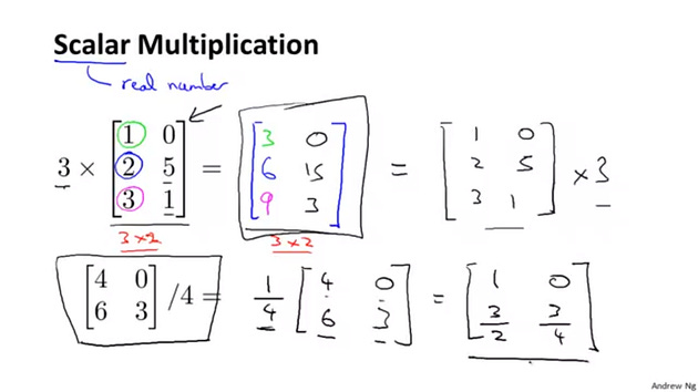
Next, let’s talk about multiplying matrices by a scalar number. And the scalar is just a, maybe a overly fancy term for, you know, a number or a real number. Alright, this means real number. So let’s take the number 3 and multiply it by this matrix. And if you do that, the result is pretty much what you’ll expect. You just take your elements of the matrix and multiply them by 3, one at a time. So, you know, one times three is three. What, two times three is six, 3 times 3 is 9, and let’s see, I’m going to stop changing colors again. Zero times 3 is zero. Three times 5 is 15, and 3 times 1 is three. And so this matrix is the result of multiplying that matrix on the left by 3. And you notice, again, this is a 3 by 2 matrix and the result is a matrix of the same dimension. This is a 3 by 2, both of these are 3 by 2 dimensional matrices. And by the way, you can write multiplication, you know, either way. So, I have three times this matrix. I could also have written this matrix and 0, 2, 5, 3, 1, right. I just copied this matrix over to the right. I can also take this matrix and multiply this by three. So whether it’s you know, 3 times the matrix or the matrix times three is the same thing and this thing here in the middle is the result. You can also take a matrix and divide it by a number. So, turns out taking this matrix and dividing it by four, this is actually the same as taking the number one quarter, and multiplying it by this matrix. 4, 0, 6, 3 and so, you can figure the answer, the result of this product is, one quarter times four is one, one quarter times zero is zero. One quarter times six is, what, three halves, about six over four is three halves, and one quarter times three is three quarters. And so that’s the results of computing this matrix divided by four.Vectors give you the result.
Section 4: Combination of Operands (Dr Andrew)

Finally, for a slightly more complicated example, you can also take these operations and combine them together. So in this calculation, I have three times a vector plus a vector minus another vector divided by three. So just make sure we know where these are, right. This multiplication. This is an example of scalar multiplication because I am taking three and multiplying it. And this is, you know, another scalar multiplication. Or more like scalar division, I guess. It really just means one zero times this. And so if we evaluate these two operations first, then what we get is this thing is equal to, let’s see, so three times that vector is three, twelve, six, plus my vector in the middle which is a 005 minus one, zero, two-thirds, right? And again, just to make sure we understand what is going on here, this plus symbol, that is matrix addition, right? I really, since these are vectors, remember, vectors are special cases of matrices, right? This, you can also call this vector addition This minus sign here, this is again a matrix subtraction, but because this is an n by 1, really a three by one matrix, that this is actually a vector, so this is also vector, this column. We call this matrix a vector subtraction, as well. OK? And finally to wrap this up. This therefore gives me a vector, whose first element is going to be 3+0–1, so that’s 3–1, which is 2. The second element is 12+0–0, which is 12. And the third element of this is, what, 6+5-(2/3), which is 11-(2/3), so that’s 10 and one-third and see, you close this square bracket. And so this gives me a 3 by 1 matrix, which is also just called a 3 dimensional vector, which is the outcome of this calculation over here. So that’s how you add and subtract matrices and vectors and multiply them by scalars or by row numbers. So far I have only talked about how to multiply matrices and vectors by scalars, by row numbers. In the next video we will talk about a much more interesting step, of taking 2 matrices and multiplying 2 matrices together.
Section 5. Practical Applications
Understanding addition and scalar multiplication of matrices has numerous practical applications in various fields. Here are a few examples:
5.1 Computer Graphics
Matrix operations play a crucial role in computer graphics for scaling, translating, and rotating objects in two-dimensional and three-dimensional spaces. Addition and scalar multiplication are used to define transformations and manipulate pixels on computer screens.
5.2 Economics
In economics, matrices are used to represent input-output models, which show how various sectors of an economy interact with each other. Addition and scalar multiplication help economists analyze changes in production levels, consumption patterns, and resource allocation.
5.3 Data Analysis
In data analysis and statistics, matrices are used to represent datasets. Addition and scalar multiplication allow analysts to perform calculations on datasets efficiently. For example, adding or subtracting matrices can help identify patterns or differences between datasets.
5.4 Physics
Matrices are extensively used in physics to describe physical systems and their interactions. Addition and scalar multiplication help physicists model complex systems, such as quantum mechanics or fluid dynamics.
Section 6- Python Implementation
import numpy as np # The swiss knife of the data scientist.
alist = [1, 2, 3, 4, 5] # Define a python list. It looks like an np array
narray = np.array([1, 2, 3, 4]) # Define a numpy array
npmatrix1 = np.array([narray, narray, narray]) # Matrix initialized with NumPy arrays
npmatrix2 = np.array([alist, alist, alist]) # Matrix initialized with lists
npmatrix3 = np.array([narray, [1, 1, 1, 1], narray]) # Matrix initialized with both types
print(npmatrix1)
print(npmatrix2)
print(npmatrix3)
okmatrix = np.array([[1, 2], [3, 4]]) # Define a 2x2 matrix
print(okmatrix) # Print okmatrix
print(okmatrix * 2) # Print a scaled version of okmatrix

# Scale by 2 and translate 1 unit the matrix
result = okmatrix * 2 + 1 # For each element in the matrix, multiply by 2 and add 1
print(result)
# Add two sum compatible matrices
result1 = okmatrix + okmatrix
print(result1)
# Subtract two sum compatible matrices. This is called the difference vector
result2 = okmatrix - okmatrix
print(result2)
result = okmatrix * okmatrix # Multiply each element by itself print(result)
Section 7. Conclusion
In conclusion, addition and scalar multiplication are fundamental operations when working with matrices. Understanding these operations is crucial for solving linear algebra problems and applying mathematical concepts to real-world scenarios. By grasping the concepts presented in this guide and exploring their practical applications, you will develop a solid foundation for further exploration of matrix operations and their significance in various disciplines.
Please Subscribe 👏Course teach for Indepth study of Machine Learning
🚀 Elevate Your Data Skills with Coursesteach! 🚀
Ready to dive into Python, Machine Learning, Data Science, Statistics, Linear Algebra, Computer Vision, and Research? Coursesteach has you covered!
🔍 Python, 🤖 ML, 📊 Stats, ➕ Linear Algebra, 👁️🗨️ Computer Vision, 🔬 Research — all in one place!
Don’t Miss Out on This Exclusive Opportunity to Enhance Your Skill Set! Enroll Today 🌟 at

Understanding of Machine Learning Course!
Artificial Intelligence Career Advice Course
Stay tuned for our upcoming articles because we research end to end , where we will explore specific topics related to Machine Learning in more detail!
🔍 Explore Tools, Python libraries for ML, Slides, Source Code, Free Machine Learning Courses from Top Universities and More!
Remember, learning is a continuous process. So keep learning and keep creating and Sharing with others!💻✌️
Note:if you are a Machine Learning export and have some good suggestions to improve this blog to share, you write comments and contribute.
if you need more update about Machine Learning and want to contribute then following and enroll in following
👉Course: Machine Learning (ML)
We offer following serveries:
We offer the following options:
Enroll in my ML course: You can sign up for the course at this link. The course is designed in a blog-style format and progresses from basic to advanced levels.
Access free resources: I will provide you with learning materials, and you can begin studying independently. You are also welcome to contribute to our community — this option is completely free.
Online tutoring: If you’d prefer personalized guidance, I offer online tutoring sessions, covering everything from basic to advanced topics. please contact:mushtaqmsit@gmail.com
Contribution: We would love your help in making coursesteach community even better! If you want to contribute in some courses , or if you have any suggestions for improvement in any coursesteach content, feel free to contact and follow.
Together, let’s make this the best AI learning Community! 🚀
Source
1- Machine Learning — Andrew