Regression Analysis Using Scikit-Learn: From Basics to Advanced Techniques

Supervised learning with scikit-learn (Part 4)

📚Chapter:2-Regression

If you want to read more articles about Supervise Learning with Sklearn, don’t forget to stay tuned :) click here.

Sections

Introduction to regression
Linear Regression
Stepwise Regression
LassoCV
ElasticNetr
RidgeCV
Polynomial regression

Description:

In this blog post, we will explore the concept of regression and its implementation using the scikit-learn library in Python. Regression is a fundamental machine learning technique used to predict continuous outcomes based on input variables. We will cover the basics of regression, different types of regression algorithms available in Scikit-learn, and provide examples of how to use them effectively. Whether you’re a beginner or an experienced data scientist, this guide will help you understand and apply regression techniques using scikit-learn.

Section 1. Introduction to regression

Now, we’re going to check out the other type of supervised learning problem: regression. In regression tasks, the target value is a continuously varying variable, such as a country’s GDP or the price of a house.

Def: Predicts continuous target variables based on input features, modeling the relationship as a linear equation.

Def :Linear regression is the fundamental supervised machine learning algorithm for predicting the continuous target variables based on the input features. As the name suggests it assumes that the relationship between the dependant and independent variable is linear. In simpler words, input features from the dataset are fed into the machine learning regression algorithm, which predicts the output values [1]

Application. It is widely used for various applications such as sales forecasting, stock market analysis, and medical research.

In scikit-learn, the linear_model module provides several regression algorithms, including linear regression, ridge regression, and lasso regression.

Regression models have many types which show below:

Section 2: Linear Regression

Def: Linear regression is one of the simplest and most widely used regression algorithms. It assumes a linear relationship between the input variables and the target variable. The goal is to find the best fit line that minimizes the sum of the squared differences between the predicted and actual values.

Scikit-learn provides the LinearRegression class to implement linear regression. We will demonstrate how to use this class with an example.

2.1- Math detail of Linear Regression

The equation of linear regression line can be represented by:

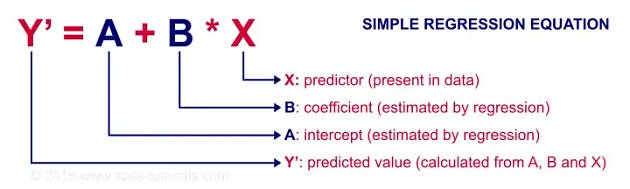
We want to fit a line to the data and a line in two dimensions is always of the form y = ax + b, where

• X = Input feature or feature matrix in multiple linear regression

• Y Predicted output (Target)

• b0 = Intercept (where the line crosses the Y-axis).

• b1 = Slope or coefficient that determines the line’s steepness.

The central idea in linear regression revolves around finding the best-fit line for our data points so that the error between the actual and predicted values is minimal. It does so by estimating the values of b0 and b1. We then utilize this line for making predictions.

a and b are the parameters of the model that we want to learn. So the question of the fitting is reduced to: how do we choose a and b? A common method is to define an error function for any given line and then to choose the line that minimizes the error function. Such an error function is also called a loss or a cost function.

The regression coefficient (m) denotes how much we expect y to change as x increases or decreases. The regression model finds the optimal values of intercept © and regression coefficient (m) such that the error (e) is minimized.

In machine learning, we use the ordinary least square method, a type of linear regression that can handle multiple input variables by minimizing the error between the actual value of y and the predicted value of y [1].

2.2- Implementation Using Scikit-Learn

Boston housing data

Our first regression task will be using the Boston housing dataset! Let’s check out the data. First, we load it from a comma-separated values file, also known as a csv file, using pandas’ read csv function. Note that you can also load this data from scikit-learn’s built-in datasets. We then view the head of the data frame using the head method. The documentation tells us the feature ‘CRIM’ is per capita crime rate, ‘NX’ is nitric oxides concentration, and ‘RM’ average number of rooms per dwelling, for example. The target variable, ‘MEDV’, is the median value of owner occupied homes in thousands of dollars.

 boston = pd.read_csv('boston.csv')
print(boston.head())

CRIM ZN INDUS CHAS NX RM AGE DIS RAD TAX \
0 0.00632 18.0 2.31 0 0.538 6.575 65.2 4.0900 1 296.0
1 0.02731 0.0 7.07 0 0.469 6.421 78.9 4.9671 2 242.0
2 0.02729 0.0 7.07 0 0.469 7.185 61.1 4.9671 2 242.0
3 0.03237 0.0 2.18 0 0.458 6.998 45.8 6.0622 3 222.0
4 0.06905 0.0 2.18 0 0.458 7.147 54.2 6.0622 3 222.0
 PTRATIO B LSTAT MEDV
0 15.3 396.90 4.98 24.0
1 17.8 396.90 9.14 21.6

Creating feature and target arrays

Now, given data as such, recall that scikit-learn wants ‘features’ and target’ values in distinct arrays, X and y,. Thus, we split our DataFrame: in the first line here, we drop the target; in the second, we keep only the target. Using the values attributes returns the NumPy arrays that we will use.

 X = boston.drop('MEDV', axis=1).values
 y = boston['MEDV'].values

Predicting house value from a single feature

As a first task, let’s try to predict the price from a single feature: the average number of rooms in a block. To do this, we slice out the number of rooms column of the DataFrame X, which is the fifth column into the variable X rooms. Checking the type of X rooms and y, we see that both are NumPy arrays. To turn them into NumPy arrays of the desired shape, we apply the reshape method to keep the first dimension, but add another dimension of size one to X.

X_rooms = X[:,5]
type(X_rooms), type(y)
(numpy.ndarray, numpy.ndarray)
y = y.reshape(-1, 1)
X_rooms = X_rooms.reshape(-1, 1)

Plotting house value vs. number of rooms

Now, let’s plot house value as a function of number of rooms using matplotlib’s plt dot scatter. We’ll also label our axes using x label and y label.

Plotting house value vs. number of rooms

We can immediately see that, as one might expect, more rooms lead to higher prices.

plt.scatter(X_rooms, y)
plt.ylabel('Value of house /1000 ($)')
plt.xlabel('Number of rooms')
plt.show();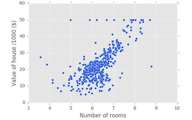

Fitting a regression model

It’s time to fit a regression model to our data. We’re going to use a model called linear regression, , I’m going to show you how to fit it and to plot its predictions. We import numpy as np, linear model from sklearn, and instantiate LinearRegression as regr. We then fit the regression to the data using regr dot fit and passing in the data, the number of rooms, and the target variable, the house price, as we did with the classification problems. After this, we want to check out the regressor’s predictions over the range of the data. We can achieve that by using np linspace between the maximum and minimum number of rooms and make a prediction for this data.

Fitting a regression model

Plotting this line with the scatter plot results in the figure you see here.

import numpy as np
from sklearn import linear_model
reg = linear_model.LinearRegression()
reg.fit(X_rooms, y)
reg.score(X, y)
# Regression coefficients
reg.coef_
reg.intercept_
prediction_space = np.linspace(min(X_rooms),
max(X_rooms)).reshape(-1, 1)
plt.scatter(X_rooms, y, color='blue')
plt.plot(prediction_space, reg.predict(prediction_space),
 ...: color='black', linewidth=3)
plt.show()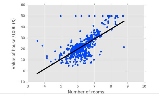

The loss function

What will our loss function be? Intuitively, we want the line to be as close to the. actual data points as possible. For this reason, we wish to minimize the vertical distance between the fit and the data. So for each data point. we calculate the vertical distance between it and the line. This distance is called a residual. Now, we could try to minimize the sum of the residuals, but then a large positive residual would cancel out.a large negative residual. For this reason we minimize the sum of the squares of the residuals! This will be our loss function and using this loss function is commonly called ordinary least squares, or OLS for short. Note that this is the same as minimizing the mean squared error of the predictions on the training set. See our statistics curriculum for more detail. When you call fit on a linear regression model in scikit-learn, it performs this OLS under the hood.

Section 3: Stepwise Regression

The stepwise regression technique is used while dealing with more than one independent variable. These variables get chosen using an automatic process without any human intervention. This is easily achievable by being observant on statistical values such as R-square, AIC metrics, and t-stats to recognize significant variables.

Scikit-learn does not have a specific implementation of stepwise regression. However, there are a few ways to perform stepwise regression in sklearn using other modules.

One way is to use the SelectKBest selector. This selector takes a scoring function as input and returns the K best features based on their scores. To perform stepwise regression, you can start with a large value of K and then iteratively reduce K and re-fit your model until you reach a satisfactory level of performance.

Another way to perform stepwise regression in sklearn is to use the RFE selector. This selector recursively eliminates features until the specified number of features remain. To perform stepwise regression, you can start with a large number of features and then iteratively eliminate features using RFE and re-fit your model until you reach a satisfactory level of performance.

Here is an example of how to perform stepwise regression in sklearn using the SelectKBest selector:

import numpy as np
import pandas as pd 
from sklearn.feature_selection import SelectKBest 
from sklearn.linear_model import LinearRegression 
# Load the data 
df = pd.read_csv('data.csv') 
# Define the target variable 
y = df['target'] 
# Define the feature variables
 X = df.drop('target', axis=1) 
# Instantiate the SelectKBest selector 
selector = SelectKBest(f_regression, k=10)
 # Fit the selector to the data 
selector.fit(X, y) 
# Get the selected features s
elected_features = selector.get_support(indices=True) 
# Create a new dataset with only the selected features
 X_selected = X[selected_features] 
# Instantiate and fit the linear regression model 
model = LinearRegression() 
model.fit(X_selected, y)

Section4- LassoCV

What is meant by LassoCV (short for “Least Absolute Shrinkage and Selection Operator”)

LassoCV regression is a supervised learning algorithm that uses cross-validation to select the optimal regularization parameter for lasso regression. LassoCV regression is a powerful tool that can be used for a variety of tasks, including feature selection, overfitting prevention, and regression. It is a good choice for situations where these factors are important.

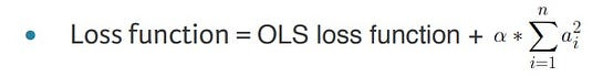
In this regression, Which our loss function is the standard OLS loss function plus the absolute value of each coefficient multiplied by some constant alpha.Linear regression can overestimate regression coefficients, adding more complexity to the machine learning model. The model becomes unstable, large, and significantly sensitive to input variables.LASSO regression is an extension of linear regression that adds a penalty (L1) to the loss function during model training to restrict (or shrink) the values of the regression coefficients. This process is known as L1 regularization [8].

L1 regularization shrinks the values of regression coefficients for input features that do not make significant contributions to the prediction task. It brings the values of such coefficient down to zero and removes corresponding input variables from the regression equation, encouraging a simpler regression model.

Lasso regression in scikit-learn

To use LassoCV regression in sklearn, you can import the LassoCV class from the linear_model module. The following code shows how to fit a LassoCV model to a dataset of house prices:

import pandas as pd
import numpy as np
import matplotlib.pyplot as plt
import seaborn as sns

data = pd.read_csv('kc_house_data.csv')
data = data.drop(['date', 'zipcode'], axis = 1)features = ['bedrooms', 'bathrooms', 'sqft_living', 'sqft_lot', 'floors', 'waterfront', 'view', 'grade', 'sqft_above', 'sqft_basement', 'condition', 'yr_built', 'yr_renovated', 'lat', 'long', 'sqft_living15', 'sqft_lot15']
X = data[features]
y = data.price
from sklearn.model_selection import train_test_split
X_train, X_test, y_train, y_test = train_test_split(X, y, test_size=0.30, random_state=0)from sklearn.linear_model import LassoCV
from sklearn.model_selection import cross_val_score
#Implementation of LassoCV
lasso = LassoCV(alphas=[0.0001, 0.001, 0.01, 0.1, 1, 10, 100])
print("Root Mean Squared Error (Lasso): ", np.sqrt(-
cross_val_score(lasso, X, y, cv=10, 
scoring='neg_mean_squared_error')).mean())
#Results
Root Mean Squared Error (Lasso):       203421.22072610114

This code will fit a lasso regression model to the data using 5-fold cross-validation. The model coefficients will then be printed to the console.

The LassoCV class has a number of parameters that can be used to control the behavior of the model. Some of the most important parameters include:

• cv: The number of folds to use in cross-validation.

• alphas: An array of regularization parameters to try.

• max_iter: The maximum number of iterations to run the solver.

• tol: The convergence tolerance.

import pandas as pd 
from sklearn.linear_model import LassoCV 
# Load the data data = pd.read_csv("house_prices.csv") 
# Split the data into features and target 
features = data.drop("price", axis=1) 
target = data["price"] 
# Fit the LassoCV model 
model = LassoCV(cv=5).fit(features, target) 
# Print the model coefficients print(model.coef_)

# Create a new house object 
new_house = {"square_feet": 1500, "bedrooms": 3, "bathrooms": 2} 
# Convert the new house object to a numpy array
 new_house_array = np.array([new_house]) 
# Make a prediction 
prediction = model.predict(new_house_array) # Print the prediction print(prediction)

Section 5- ElasticNet

What is ElasticNet Regression

Elastic Net Regression is a powerful machine learning algorithm that combines the features of both Lasso and Ridge Regression. It is a regularized regression technique that is used to deal with the problems of multicollinearity and overfitting, which are common in high-dimensional datasets. This algorithm works by adding a penalty term to the standard least-squares objective function [7].

Elastic Net Regression was introduced by Zou and Hastie in 2005. It is a linear regression algorithm that adds two penalty terms to the standard least-squares objective function. These two penalty terms are the L1 and L2 norms of the coefficient vector, which are multiplied by two hyperparameters, alpha and lambda. The L1 norm is used to perform feature selection, whereas the L2 norm is used to perform feature shrinkage [7].

The Elastic Net Regression model can be represented as follows :

y = b0 + b1*x1 + b2*x2 + … + bn*xn + e

Where y is the dependent variable, b0 is the intercept, b1 to bn are the regression coefficients, x1 to xn are the independent variables, and e is the error term. The Elastic Net Regression model tries to minimize the following objective function:

RSS + λ * [(1 - α) * ||β||2 + α * ||β||1]

Where RSS is the residual sum of squares, λ is the regularization parameter, β is the coefficient vector, α is the mixing parameter between the L1 and L2 norms, ||β||2 is the L2 norm of β, and ||β||1 is the L1 norm of β.

Elastic Net Regression in Python

Elastic net regression is implemented in the scikit-learn library for Python using the ElasticNet class. The ElasticNet class has two main hyperparameters:

• alpha: Controls the overall strength of the regularization penalty. A larger value of alpha will result in more shrinkage of the coefficients.

• l1_ratio: Controls the balance between the L1 and L2 regularization penalties. A value of l1_ratio=1 corresponds to pure lasso regularization, while a value of l1_ratio=0 corresponds to pure ridge regularization.

The following code shows how to use the ElasticNet class to fit a model to a dataset of house prices:

from sklearn.linear_model import ElasticNet 
# Load the data data = pd.read_csv("house_prices.csv") 
# Split the data into features and target 
features = data.drop("price", axis=1)
target = data["price"]
 # Fit the ElasticNet model 
model = ElasticNet(alpha=1.0, l1_ratio=0.5).fit(features, target) 
# Print the model coefficients 
print(model.coef_)

from sklearn.linear_model import LassoCV, RidgeCV, ElasticNet
from sklearn.model_selection import cross_val_score
#Implementation of ElasticNet
elastic = ElasticNet(alpha=0.001)
print("Root Mean Squared Error (ElasticNet): ", np.sqrt(-cross_val_score(elastic, X, y, cv=10, scoring='neg_mean_squared_error')).mean())

Section-6- Ridge regression

What is meant by Ridge regression?

Ridge regression is a type of linear regression that adds a regularization term to the cost function, which helps to reduce the variance of the model and improve its performance on unseen data. In Rdige regression, which our loss function is the standard OLS loss function plus the squared value of each coefficient multiplied by some constant alpha. Thus, when minimizing the loss function to fit to our data, models are penalized for coefficients with a large magnitude: large positive and large negative coefficients, that is. Note that alpha is a parameter we need to choose in order to fit and predict. Essentially, we can select the alpha for which our model performs best. Picking alpha for ridge regression is similar to picking k in KNN.

This is called hyperparameter tuning and we’ll see much more of this soon. This alpha, which you may also see called lambda in the wild, can be thought of as a parameter that controls model complexity. Notice that when alpha is equal to zero, we get back OLS. Large coefficients in this case are not penalized and the overfitting problem is not accounted for. A very high alpha means that large coefficients are significantly penalized, which can lead to a model that is too simple and ends up underfitting the data. The method of performing ridge regression with scikit-learn mirrors the other models that we have seen [8].

Ridge regression is another regularized machine learning algorithm that adds an L2 regularization penalty to the loss function during the model training phase. Like lasso, ridge regression also minimizes multicollinearity, which occurs when multiple independent variables show a high correlation with each other.[1]. L2 regularization deals with multicollinearity by minimizing the effects of such independent variables, reducing the values of corresponding regression coefficients close to zero. Unlike L1 regularization, it prevents the complete removal of any variable.[1] The following code snippet implements ridge regression using the scikit-learn library. In scikit-learn, the L2 penalty is weighted by the alpha hyperparameter.[8]

Why regularize?

what fitting a linear regression does is minimize a loss function to choose a coefficient ai for each feature variable. If we allow these coefficients or parameters to be super large, we can get overfitting. It isn’t so easy to see in two dimensions, but when you have loads and loads of features, that is, if your data sit in a high-dimensional space with large coefficients, it gets easy to predict nearly anything. For this reason, it is common practice to alter the loss function so that it penalizes for large coefficients. This is called regularization. The first type of regularized regression that we’ll look at is called ridge regression [1]

Advantages

• RidgeCV is a convenient way to tune the hyperparameter alpha of ridge regression without having to manually perform cross-validation. It is also a good choice for datasets with a large number of features, as it can help to prevent overfitting.

Ridge regression in scikit-learn

RidgeCV is a class in the scikit-learn Python library that implements ridge regression with built-in cross-validation.RidgeCV works by first splitting the training data into multiple folds. Then, it trains a ridge regression model on each fold, using a different value of the regularization parameter alpha for each model. Finally, it selects the model with the best performance on the cross-validation folds as the final model.

We import Ridge from sklearn dot linear model, we split our data into test and train, fit on the training, and predict on the test. Note that we set alpha using the keyword argument alpha. Also notice the argument normalize: setting this equal to True ensures that all our variables are on the same scale and we will cover this in more depth later. There is another type of regularized regression called lasso regression [1],

from sklearn.linear_model import RidgeCV
from sklearn.model_selection import cross_val_score
 # Load the training data 

X = np.array([[1, 1], [1, 2], [1, 3], [2, 1], [2, 2], [2, 3]])
y = [ 6, 8, 10, 7, 9, 11]

# Create a RidgeCV object 
clf = RidgeCV(alphas=[0.0001, 0.001, 0.01, 0.1, 1, 10, 100],normalize=True)
# Fit the model
 clf.fit(X, y) 
# Make predictions on new data 
y_pred = clf.predict(X_new)
# Performance
print("Root Mean Squared Error (Ridge): ", np.sqrt(-cross_val_score(ridge, X, y, cv=10, scoring='neg_mean_squared_error')).mean())
# Regression coefficients
clf.coef
clf.intercept_

Section 7-Polynomial regression

Polynomial regression is a type of regression analysis in which the relationship between the independent variable x and the dependent variable y is modeled as an nth-degree polynomial. This means that the relationship is not a straight line, but instead a curve. Polynomial regression is a useful tool for modeling relationships that are not linear, but it is important to note that it can be overfitted easily.

To perform polynomial regression with sklearn, you will need to use the PolynomialFeatures and LinearRegression modules. The PolynomialFeatures module will create new features by raising the original features to a power. The LinearRegression module will then fit a linear regression model to these new features.

Here is an example of how to perform polynomial regression with sklearn:

import pandas as pd
import numpy as np
from sklearn.linear_model import LinearRegression
from sklearn.preprocessing import PolynomialFeatures
from sklearn.model_selection import train_test_split
from sklearn.metrics import mean_squared_error
data = pd.read_csv('data.csv')

X = data[['feature1', 'feature2']]
y = data['target_variable']

#Split the data into training and testing sets:
X_train, X_test, y_train, y_test = train_test_split(X, y, test_size=0.2)
# Create a polynomial features object
poly = PolynomialFeatures(degree=2)
X_train_poly = poly.fit_transform(X_train)
X_test_poly = poly.transform(X_test)
# Create a linear regression object:
model = LinearRegression()
model.fit(X_train_poly, y_train)
y_pred = model.predict(X_test_poly)
mse = mean_squared_error(y_test, y_pred)
print('MSE:', mse)

Please Subscribe 👏Course teach for Indepth study of Supervised Learning with Sklearn

🚀 Elevate Your Data Skills with Coursesteach! 🚀

Ready to dive into Python, Machine Learning, Data Science, Statistics, Linear Algebra, Computer Vision, and Research? Coursesteach has you covered!

🔍 Python, 🤖 ML, 📊 Stats, ➕ Linear Algebra, 👁️‍🗨️ Computer Vision, 🔬 Research — all in one place!

Enroll now for top-tier content and kickstart your data journey!

Supervised learning with scikit-learn

🔍 Explore cutting-edge tools and Python libraries, access insightful slides and source code, and tap into a wealth of free online courses from top universities and organizations. Connect with like-minded individuals on Reddit, Facebook, and beyond, and stay updated with our YouTube channel and GitHub repository. Don’t wait — enroll now and unleash your ML with Sklearn potential!”

Stay tuned for our upcoming articles because we reach end to end ,where we will explore specific topics related to Supervised learning with sklearn in more detail!

Remember, learning is a continuous process. So keep learning and keep creating and Sharing with others!💻✌️

We offer following serveries:
We offer the following options:

1. Enroll in my ML Libraries course: You can sign up for the course at this link. The course is designed in a blog-style format and progresses from basic to advanced levels.

2. Access free resources: I will provide you with learning materials, and you can begin studying independently. You are also welcome to contribute to our community — this option is completely free.

3. Online tutoring: If you’d prefer personalized guidance, I offer online tutoring sessions, covering everything from basic to advanced topics. please contact:mushtaqmsit@gmail.com

Contribution: We would love your help in making coursesteach community even better! If you want to contribute in some courses , or if you have any suggestions for improvement in any coursesteach content, feel free to contact and follow.

Together, let’s make this the best AI learning Community! 🚀

👉📚GitHub Repository

Together, let’s make this the best AI learning Community! 🚀

👉WhatsApp

👉 Facebook

👉Github

👉LinkedIn

👉Youtube

👉Twitter

Source

1- Introduction to Linear regression

2- The basic of linear regression

3–Machine Learning with scikit-learning (Datacamp)

4-Hands-On with Supervised Learning: Linear Regression

5-Top 6 Regression Techniques a Data Science Specialist Needs to Know

6–Introduction to Linear Regression — mathematics and application with Python

7–1-Elastic Net Regression detailed guide!

8–Machine Learning with scikit-learning (Datacamp)