PyCaret Anomaly Detection with a Simple Python

PyCaret (Part 4)

📚Chapter: — PyCaret

If you want to read more articles about Machine Learning Libraries , don’t forget to stay tuned :) click here.

Introduction

In this blog post, we will explore how to perform anomaly detection using PyCaret, a low-code machine learning library in Python. Anomaly detection is an important task for identifying unusual patterns or outliers in data, which can indicate fraud, defects, or other unusual behavior. We will also work with the 'BULLETIN' dataset to demonstrate the process.

What is mean by Anomaly Detection

Anomaly detection refers to identifying data points that deviate significantly from the normal patterns or trends within the dataset. These data points, often referred to as outliers, can indicate rare but potentially important events, such as fraudulent transactions, system failures, or rare medical conditions.

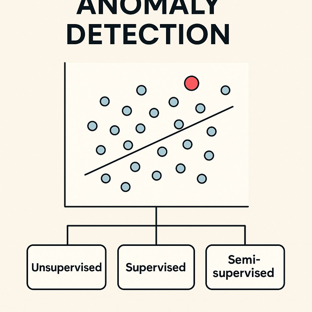
Anomaly Detection is the task of identifying the rare items, events or observations which raise suspicions by differing significantly from the majority of the data. Typically, the anomalous items will translate to some kind of problem such as bank fraud, a structural defect, medical problems or errors in a text. There are three broad categories of anomaly detection techniques exist:

• Unsupervised anomaly detection: Unsupervised anomaly detection techniques detect anomalies in an unlabeled test data set under the assumption that the majority of the instances in the dataset are normal by looking for instances that seem to fit least to the remainder of the data set.

• Supervised anomaly detection: This technique requires a dataset that has been labeled as "normal" and "abnormal" and involves training a classifier.

• Semi-supervised anomaly detection: This technique constructs a model representing normal behavior from a given normal training dataset, and then tests the likelihood of a test instance to be generated by the learnt model.

Why PyCaret for Anomaly Detection?

PyCaret provides a simple interface for performing machine learning tasks, including anomaly detection, with minimal code. It integrates various models and allows users to experiment with them using only a few lines of code. The library also handles preprocessing, model comparison, and evaluation in an automated way.

pycaret.anomaly module supports the unsupervised and supervised anomaly detection techniques. In this tutorial, we will only cover unsupervised anomaly detection techniques.

PyCaret's anomaly detection module (pycaret.anomaly) is a an unsupervised machine learning module which performs the task of identifying rare items, events or observations which raise suspicions by differing significantly from the majority of the data.

PyCaret anomaly detection module provides several pre-processing features that can be configured when initializing the setup through setup() function. It has over 12 algorithms and few plots to analyze the results of anomaly detection. PyCaret's anomaly detection module also implements a unique function tune_model() that allows you to tune the hyperparameters of anomaly detection model to optimize the supervised learning objective such as AUC for classification or R2 for regression.

Steps for Anomaly Detection in PyCaret

1. Install PyCaret

2. Load and prepare the data

3. Set up the PyCaret environment

4. Run anomaly detection models

5. Evaluate the results

Let’s go step-by-step through the implementation.

Step 1: Install PyCaret

To get started, we first need to install PyCaret. You can install it via pip:

Import library

import numpy as np 
import pandas as pd 
import seaborn as sns 
import matplotlib.pyplot as plt
from prettytable import PrettyTable
from sklearn.model_selection import train_test_split
import warnings
warnings.filterwarnings("ignore")
#from pycaret.utils import enable_colab
#enable_colab()

Installing PyCaret

The first step to getting started with PyCaret is to install PyCaret. Installing PyCaret is easy and takes few minutes only. Follow the instructions below:

Installing PyCaret in Colab

#capture #suppresses the displays
# install the full version
!pip install pycaret[full]

!pip install pyyaml==5.4.1

For Google colab users

from pycaret.utils import enable_colab
enable_colab()

Import the necessary packages

!pip install markupsafe==2.0.1

Runtime> Restart Runtime

import pandas as pd
import numpy as np
import matplotlib.pyplot as plt
import seaborn as sns
import pycaret
import jinja2

Steps 2- Load and Prepare the Dataset

For this tutorial, we will use a dataset from UCI called Mice Protein Expression. The dataset consists of the expression levels of 77 proteins/protein modifications that produced detectable signals in the nuclear fraction of cortex. The dataset contains a total of 1080 measurements per protein. Each measurement can be considered as an independent sample/mouse. Click Here to read more about the dataset.

You can download the data from the original source found here and load it using pandas (Learn How) or you can use PyCaret's data respository to load the data using get_data() function (This will require internet connection).

from pycaret.datasets import get_data
dataset = get_data('mice')

#check the shape of data
dataset.shape

In order to demonstrate the predict_model() function on unseen data, a sample of 5% (54 samples) are taken out from original dataset to be used for predictions at the end of experiment. This should not be confused with train/test split. This particular split is performed to simulate real life scenario. Another way to think about this is that these 54 samples are not available at the time when this experiment was performed.

data = datasets.sample(frac=0.95, random_state=786)
data_unseen = datasets.drop(data.index)

data.reset_index(drop=True, inplace=True)
data_unseen.reset_index(drop=True, inplace=True)

print('Data for Modeling: ' + str(data.shape))
print('Unseen Data For Predictions: ' + str(data_unseen.shape))

Step 3: Set Up the PyCaret Environment

setup() function initializes the environment in PyCaret and creates the transformation pipeline to prepare the data for modeling and deployment. setup() must be called before executing any other function in PyCaret. It takes only one mandatory parameter: pandas dataframe. All other parameters are optional and are used to customize pre-processing pipeline .

When setup() is executed, PyCaret's inference algorithm will automatically infer the data types for all features based on certain properties. Although, most of the times the data type is inferred correctly but it's not always the case. Therefore, after setup() is executed, PyCaret displays a table containing features and their inferred data types. At which stage, you can inspect and press enter to continue if all data types are correctly inferred or type quit to end the experiment. Identifying data types correctly is of fundamental importance in PyCaret as it automatically performs few pre-processing tasks which are imperative to perform any machine learning experiment. These pre-processing tasks are performed differently for each data type. As such, it is very important that data types are correctly configured.

from pycaret.anomaly import *
exp_ano101 = setup(data, normalize = True,  ignore_features = ['MouseID'], session_id = 123)

Once the setup is succesfully executed it prints the information grid that contains few important information. Much of the information is related to pre-processing pipeline which is constructed when setup() is executed. Much of these features are out of scope for the purpose of this tutorial. However, few important things to note at this stage are:

• session_id : A pseudo-random number distributed as a seed in all functions for later reproducibility. If no session_id is passed, a random number is automatically generated that is distributed to all functions. In this experiment session_id is set as 123 for later reproducibility.

• We specify normalize=True to scale the data, which is often important for anomaly detection.

• Missing Values : When there are missing values in original data it will show as True. Notice that Missing Values in the information grid above is True as the data contains missing values which are automatically imputed using mean for numeric features and constant for categorical features. The method of imputation can be changed using numeric_imputation and categorical_imputation parameter in setup().

• Original Data : Displays the original shape of dataset. In this experiment (1026, 82) means 1026 samples and 82 features.

• Transformed Data : Displays the shape of transformed dataset. Notice that the shape of original dataset (1026, 82) is transformed into (1026, 91). The number of features has increased due to encoding of categorical features in the dataset.

• Numeric Features : Number of features inferred as numeric. In this dataset, 77 out of 82 features are inferred as numeric.

• Categorical Features : Number of features inferred as categorical. In this dataset, 5 out of 82 features are inferred as categorical. Also notice, we have ignored one categorical feature i.e. MouseID using ignore_feature parameter.

Notice that how few tasks such as missing value imputation and categorical encoding that are imperative to perform modeling are automatically handled. Most of the other parameters in setup() are optional and used for customizing pre-processing pipeline. These parameters are out of scope for this tutorial but as you progress to intermediate and expert level, we will cover them in much detail.

Step 4: Run Anomaly Detection Models

Once the environment is set up, we can run the anomaly detection models using the create_model() function. PyCaret offers several algorithms for anomaly detection, such as iforest (Isolation Forest), lof (Local Outlier Factor), and knn (K-Nearest Neighbors).

Creating an anomaly detection model in PyCaret is simple and similar to how you would have created a model in supervised modules of PyCaret. The anomaly detection model is created using create_model() function which takes one mandatory parameter i.e. name of the model as a string. This function returns a trained model object. See the example below:

iforest = create_model('iforest')

print(iforest)

We have created Isolation Forest model using create_model(). Notice the contamination parameter is set 0.05 which is the default value when you do not pass fraction parameter in create_model(). fraction parameter determines the proportion of outliers in the dataset. In below example, we will create One Class Support Vector Machine model with 0.025 fraction.

svm = create_model('svm', fraction = 0.025)

print(svm)

Just by replacing iforest with svm inside create_model() we have now created OCSVM anomaly detection model. There are 12 models available ready-to-use in pycaret.anomaly module. To see the complete list, please see docstring or use models function.

models()

You can also compare different models and select the best one for your dataset:

# Compare all models for anomaly detection
best_model = compare_models()

Steps 5- Assign a Model

Now that we have created a model, we would like to assign the anomaly labels to our dataset (1080 samples) to analyze the results. We will achieve this by using assign_model() function. See an example below:

iforest_results = assign_model(iforest)
iforest_results.head()

Notice that two columns Label and Score are added towards the end. 0 stands for inliers and 1 for outliers/anomalies. Score is the values computed by the algorithm. Outliers are assigned with larger anomaly scores. Notice that iforest_results also includes MouseID feature that we have dropped during setup(). It wasn't used for the model and is only appended to the dataset when you use assign_model(). In the next section we will see how to analyze the results of anomaly detection using plot_model().

Step 5: Evaluate the Results

Steps 6- Plot a Model

plot_model() function can be used to analyze the anomaly detection model over different aspects. This function takes a trained model object and returns a plot. See the examples below:

T-distributed Stochastic Neighbor Embedding (t-SNE)

plot_model(iforest)

plot_model(iforest, plot = 'tsne')

plot_model(iforest, plot = 'umap')

Steps 7- Predict on Unseen Data

predict_model() function is used to assign anomaly labels on the new unseen dataset. We will now use our iforest model to predict the data stored in data_unseen. This was created in the beginning of the experiment and it contains 54 new samples that were not exposed to PyCaret before.

unseen_predictions = predict_model(iforest, data=data_unseen)
unseen_predictions.head()

Label column indicates the outlier (1 = outlier, 0 = inlier). Score is the values computed by the algorithm. Outliers are assigned with larger anomaly scores. You can also use predict_model() function to label the training data. See example below:

data_predictions = predict_model(iforest, data = data)
data_predictions.head()

Steps 8- Saving the Model

We have now finished the experiment by using our iforest model to predict outlier labels on unseen data. This brings us to the end of our experiment but one question is still to be asked. What happens when you have more new data to predict? Do you have to go through the entire experiment again? The answer is No, you don't need to rerun the entire experiment and reconstruct the pipeline to generate predictions on new data. PyCaret's inbuilt function save_model() allows you to save the model along with entire transformation pipeline for later use.

save_model(iforest,'Final IForest Model 25Nov2020')

Loading the Saved Model

To load a saved model on a future date in the same or different environment, we would use the PyCaret's load_model() function and then easily apply the saved model on new unseen data for prediction

saved_iforest = load_model('Final IForest Model 25Nov2020')

Once the model is loaded in the environment, you can simply use it to predict on any new data using the same predict_model() function . Below we have applied the loaded model to predict the same data_unseen that we have used in section 10 above.

new_prediction = predict_model(saved_iforest, data=data_unseen)

new_prediction.head()

Notice that results of unseen_predictions and new_prediction are identical.

Please Follow and 👏 Subscribe for the story courses teach to see latest updates on this story

🚀 Elevate Your Data Skills with Coursesteach! 🚀

Ready to dive into Python, Machine Learning, Data Science, Statistics, Linear Algebra, Computer Vision, and Research? Coursesteach has you covered!

🔍 Python, 🤖 ML, 📊 Stats, ➕ Linear Algebra, 👁️‍🗨️ Computer Vision, 🔬 Research — all in one place!

Don’t Miss Out on This Exclusive Opportunity to Enhance Your Skill Set! Enroll Today 🌟 at

Machine Learning libraries Course

🔍 Explore Tools, Python libraries for ML, Slides, Source Code, Free online Courses and More!

Stay tuned for our upcoming articles because we reach end to end ,where we will explore specific topics related to Machine Learning libraries in more detail!

Remember, learning is a continuous process. So keep learning and keep creating and Sharing with others!💻✌️

Ready to dive into data science and AI but unsure how to start? I’m here to help! Offering personalized research supervision and long-term mentoring. Let’s chat on Skype: themushtaq48 or email me at mushtaqmsit@gmail.com. Let’s kickstart your journey together!

Contribution: We would love your help in making coursesteach community even better! If you want to contribute in some courses , or if you have any suggestions for improvement in any coursesteach content, feel free to contact and follow.

Together, let’s make this the best AI learning Community! 🚀

👉WhatsApp

👉 Facebook

👉Github

👉LinkedIn

👉Youtube

👉Twitter

References

1- Anomaly Detection Tutorial (ANO101) - Level Beginner

2-Getting familiar with PyCaret for anomaly detection