


NumPy Basics Guide: Efficient Array Operations for Python Data Science
ML- Libraries (Part 4)

📚Chapter: 1 - NumPy
If you want to read more articles about Machine Learning Libraries , don’t forget to stay tuned :) click here.
Introduction
NumPy, short for Numerical Python, is a fundamental library in the Python programming language for performing numerical operations efficiently. At the core of NumPy is the ndarray, a multi-dimensional array that provides a flexible and efficient container for large datasets. In this blog post, we’ll delve into the basics of NumPy array operations, exploring essential functions that make NumPy a powerhouse for scientific computing and data analysis.

NumPy’s main object is the homogeneous multidimensional array. It is a table of elements (usually numbers), all of the same type, indexed by a tuple of non-negative integers. In NumPy dimensions are called axes. For example, the array for the coordinates of a point in 3D space, [1, 2, 1], has one axis. That axis has 3 elements in it, so we say it has a length of 3. In the example pictured below, the array has 2 axes. The first axis has a length of 2, the second axis has a length of 3. [[1., 0., 0.], [0., 1., 2.]] NumPy’s array class is called ndarray. It is also known by the alias array. Note that numpy.array is not the same as the Standard Python Library class array.array, which only
Sections
Array Inspection
indexing and Slicing
Aggregation Functions
Reshaping and Transposing
Append and Delete
Conclusion
Section 1- Array Shape and Size:
Understanding the shape and size of an array is crucial. You can obtain this information using the shape and size attributes:
1- ndarray.ndim
the number of axes (dimensions) of the array.
2-ndarray.shape
Array shape specifies the number of elements along each dimension.the dimensions of the array. This is a tuple of integers indicating the size of the array in each dimension. For a matrix with n rows and m columns, shape will be (n,m). The length of the shape tuple is therefore the number of axes, ndim.
3- ndarray.size
Array size is basically the product of a number of rows and columns.
4- ndarray.dtype
an object describing the type of the elements in the array. One can create or specify dtype’s using standard Python types. Additionally NumPy provides types of its own. numpy.int32, numpy.int16, and numpy.float64 are some examples.
5-ndarray.itemsize
the size in bytes of each element of the array. For example, an array of elements of type float64 has itemsize 8 (=64/8), while one of type complex32 has itemsize 4 (=32/8). It is equivalent to ndarray.dtype.
6- itemsize.
ndarray.data the buffer containing the actual elements of the array. Normally, we won’t need to use this attribute because we will access the elements in an array using indexing facilities.
Example
arr = np.arange(15).reshape(3, 5)
# Arange function will create 15 points from 0 to 14 and then reshape will reshape it accordingly
print(arr.shape)
print(arr.ndim)
print(arr.dtype.name)
print(arr.size)
print(type(arr))Section 2- Indexing and Slicing
NumPy supports powerful indexing and slicing operations for extracting specific elements or subarrays from an array: Array indexing Refers to accessing individual elements within a NumPy array,.Array Slicing: This allows you to extract specific portions of an array, creating new arrays with the selected elements.
We can index and slice NumPy arrays in all the ways we can slice python lists [1]:
# Accessing a specific element
specific_element = arr_2d[1, 2]
# Slicing a subarray
subarray = arr_1d[1:4]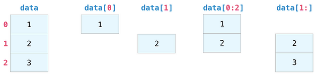
# Creating a NumPy array
arr = np.array([10, 20, 30, 40, 50])
# Accessing individual elements
first_element = arr[0] # Access the first element (10)
# Accessing elements using negative indices
last_element = arr[-1] # Access the last element (50)
# Creating a 2D NumPy array
arr_2d = np.array([[1, 2, 3], [4, 5, 6], [7, 8, 9]])
# Slicing along rows and columns
sliced_array = arr_2d[0,1] # Element at row 0, column 1 (value: 2)
# Slicing the array to create a new array
sliced_array = arr[1:4] # Slice from index 1 to 3 (exclusive) [20,30,40]
# Slicing with a step of 2
sliced_array = arr[0::2] # Start at index 0, step by 2 [10,30,50]
# Slicing with negative index
second_to_last = arr[-2::] # Access the last two elements [40,50]
# Conditional slicing: Select elements greater than 30
sliced_array = arr[arr > 30] # Result: [40, 50]
# Creating a 2D NumPy array
arr_2d = np.array([[1, 2, 3], [4, 5, 6], [7, 8, 9]])
# Slicing along rows and columns
sliced_array = arr_2d[1:3, 0:2] # Slice a 2x2 subarray: [[4, 5], [7, 8]]Section 3- Aggregation Functions
NumPy provides functions for aggregating data, such as calculating the sum, mean, minimum, and maximum:
in addition to min, max, and sum, you get all the greats like mean to get the average, prod to get the result of multiplying all the elements together, std to get standard deviation, and plenty of others [4].

# Calculating the sum of an array
sum_of_array = np.sum(arr_2d)
# Calculating the mean of an array
mean_of_array = np.mean(arr_1d)
# Finding the minimum and maximum values in an array
min_value = np.min(arr_2d)
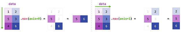
max_value = np.max(arr_1d)We can aggregate matrices the same way we aggregated vectors [4]:

import numpy as np# Creating a 2D array
matrix = np.array([[1, 2, 3], [4, 5, 6], [7, 8, 9]])
print(matrix)
# Sum of all elements
total_sum = np.sum(matrix)
print("Total Sum:", total_sum)
# Sum along each column (axis=0)
column_sums = np.sum(matrix, axis=0)
print("Column Sums:", column_sums)
# Sum along each row (axis=1)
row_sums = np.sum(matrix, axis=1)
print("Row Sums:", row_sums)2. Mean and Average:
# Mean of all elements
mean_value = np.mean(matrix)
print("Mean:", mean_value)
# Mean along each column
column_means = np.mean(matrix, axis=0)
print("Column Means:", column_means)# Mean along each row
row_means = np.mean(matrix, axis=1)
print("Row Means:", row_means)3. Maximum and Minimum:
# Maximum element
max_value = np.max(matrix)
print("Maximum Value:", max_value)
# Maximum along each column
column_max = np.max(matrix, axis=0)
print("Column Max Values:", column_max)# Maximum along each row
row_max = np.max(matrix, axis=1)
print("Row Max Values:", row_max)# Minimum element
min_value = np.min(matrix)
print("Minimum Value:", min_value)Not only can we aggregate all the values in a matrix, but we can also aggregate across the rows or columns by using the axis parameter [4]:
Section 4- Reshaping and Transposing
You can change the shape of an array using the reshape function:
In more advanced use case, you may find yourself needing to switch the dimensions of a certain matrix. This is often the case in machine learning applications where a certain model expects a certain shape for the inputs that is different from your dataset. NumPy’s reshape() method is useful in these cases. You just pass it the new dimensions you want for the matrix. You can pass -1 for a dimension and NumPy can infer the correct dimension based on your matrix [4]:

# Reshaping a 1D array into a 2D array
reshaped_array = arr_1d.reshape((5, 1))
import numpy as np# Creating a 1D array with 12 elements
data = np.arange(1, 13)
print("Original 1D array:\n", data)Reshaping 1D Array to 2D Array:
import numpy as np

# Creating a 1D array
original_array = np.array([1, 2, 3, 4, 5, 6, 7, 8, 9])

# Reshaping the 1D array to a 2D array with 3 rows and 3 columns
reshaped_array = original_array.reshape(3, 3)

# Printing the original and reshaped arrays
print("Original 1D array:")
print(original_array)
print("\nReshaped 2D array:")
print(reshaped_array)
In this example, we first create a 1D array named original_array with 9 elements. We then use the reshape function to reshape it into a 2D array with 3 rows and 3 columns ((3, 3)). The reshaped array is stored in the variable reshaped_array. Finally, we print both the original and reshaped arrays.
You can adjust the dimensions passed to the reshape function according to your needs. It's important to note that the total number of elements in the original array must be equal to the product of the dimensions specified for the reshaped array.
Reshaping 1D Array to 3D Array:
import numpy as np

# Creating a 1D array
original_array = np.array([1, 2, 3, 4, 5, 6, 7, 8, 9, 10, 11, 12])

# Reshaping the 1D array to a 3D array with 2 blocks, 2 rows, and 3 columns
reshaped_array = original_array.reshape(2, 2, 3)

# Printing the original and reshaped arrays
print("Original 1D array:")
print(original_array)
print("\nReshaped 3D array:")
print(reshaped_array)
Reshaping with -1:
The use of -1 in the reshape function allows NumPy to automatically calculate the size of that dimension. This is particularly useful when you want to maintain a specific number of elements without explicitly specifying the size of one dimension:
import numpy as np

# Creating a 1D array with 12 elements
original_array = np.array([1, 2, 3, 4, 5, 6, 7, 8, 9, 10, 11, 12])

# Reshaping the 1D array to a 2D array with 4 rows and an automatically calculated number of columns
reshaped_array = original_array.reshape(-1, 4)

# Printing the original and reshaped arrays
print("Original 1D array:")
print(original_array)
print("\nReshaped 2D array with -1:")
print(reshaped_array)
Flattening a 2D or 3D Array:
Flattening is the process of converting a multi-dimensional array into a 1D array. The flatten method achieves this:
import numpy as np

# Creating a 2D array
original_2d_array = np.array([[1, 2, 3], [4, 5, 6], [7, 8, 9]])

# Flattening the 2D array using flatten()
flattened_array = original_2d_array.flatten()

# Printing the original and flattened arrays
print("Original 2D array:")
print(original_2d_array)
print("\nFlattened 1D array:")
print(flattened_array)
import numpy as np
# Creating a 3D array
original_3d_array = np.array([[[1, 2], [3, 4]], [[5, 6], [7, 8]], [[9, 10], [11, 12]]])
# Flattening the 3D array using flatten()
flattened_array_3d = original_3d_array.flatten()
# Printing the original and flattened arrays
print("Original 3D array:")
print(original_3d_array)
print("\nFlattened 1D array:")
print(flattened_array_3d)A common need when dealing with matrices is the need to rotate them. This is often the case when we need to take the dot product of two matrices and need to align the dimension they share. NumPy arrays have a convenient property called T to get the transpose of a matrix [4]:

In linear algebra, the transpose of a matrix is an operator that flips a matrix over its diagonal, i.e., the transpose operator switches the row and column indices of the matrix producing another matrix. If the original matrix dimension is n by m, the resulting transposed matrix will be m by n.
T denotes the transpose operations with NumPy matrices.
matrix3x2 = np.array([[1, 2], [3, 4], [5, 6]]) # Define a 3x2 matrix
print('Original matrix 3 x 2')
print(matrix3x2)
print('Transposed matrix 2 x 3')
print(matrix3x2.T)
Original matrix 3 x 2
[[1 2]
[3 4]
[5 6]]
Transposed matrix 2 x 3
[[1 3 5]
[2 4 6]]However, note that the transpose operation does not affect 1D arrays.
nparray = np.array([1, 2, 3, 4]) # Define an array
print('Original array')
print(nparray)
print('Transposed array')
print(nparray.T)
Original array
[1 2 3 4]
Transposed array
[1 2 3 4]perhaps in this case you wanted to do:
nparray = np.array([[1, 2, 3, 4]]) # Define a 1 x 4 matrix. Note the 2 level of square brackets
print('Original array')
print(nparray)
print('Transposed array')
print(nparray.T)
Original array
[[1 2 3 4]]
Transposed array
[[1]
[2]
[3]
[4]]Section 5- Append and Delete
To append arrays in NumPy, you can use the numpy.append() function. This function allows you to add elements to the end of an existing array along a specified axis. Keep in mind that np.append() returns a new array with the appended elements; so it does not modify the original arrays. If you want to modify an existing array in-place, you can use methods like np.concatenate() or use assignment statements. we can use np.delete to remove the items from an array [3].
# Create an array
original_array = np.array([1, 2, 3])
# Append elements in-place
original_array = np.append(original_array, [4, 5, 6])
# Create a NumPy array
arr = np.array([1, 2, 3, 4, 5])
# Remove the item at index 2 (value 3)
new_arr = np.delete(arr, 2)
# Create a 2D NumPy array
arr = np.array([[1, 2, 3], [4,5, 6], [7, 8, 9]])
# Remove the second row (index 1)
new_arr = np.delete(arr, 1, axis=0)
Conclusion:
Understanding the basics of NumPy array operations is fundamental for anyone working with scientific computing and data analysis in Python. The ability to perform efficient element-wise operations, manipulate array shapes, and aggregate data easily makes NumPy a go-to tool for numerical tasks. As you delve deeper into the world of NumPy, you’ll discover more advanced operations and functionalities that contribute to its versatility in the realm of scientific computing.
Please Subscribe courses teach to learn about Machine Learning libraries
If you want to learn more about these topics: Python, Machine Learning Data Science, Statistic For Machine learning, Linear Algebra for Machine learning Computer Vision and Research
Then Login and Enroll in Coursesteach to get fantastic content in the data field.
Stay tuned for our upcoming articles where we will explore specific topics related to Machine Learning in more detail!
Remember, learning is a continuous process. So keep learning and keep creating and Sharing with others!💻✌️
Note:if you are a Machine Learning export and have some good suggestions to improve this blog to share, you write comments and contribute.
if you need more update about Machine Learning and want to contribute then following and enroll in following
👉Course: Machine Learning Libraries
Contribution: We would love your help in making coursesteach community even better! If you want to contribute in some courses , or if you have any suggestions for improvement in any coursesteach content, feel free to contact and follow.
Together, let’s make this the best AI learning Community! 🚀
Source
1- A Visual Intro to NumPy and Data Representation