


Linear Regression Simplified: Exploring Cost Function with One Variable
ML(P-6)

📚Chapter:2-Regression
If you want to read more articles about Supervise Learning with Sklearn, don’t forget to stay tuned :) click here.
What the cost function is doing?
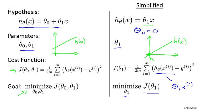
We want to fit a straight line to our data, so we had this formed as a hypothesis with these parameters theta zero and theta one, and with different choices of the parameters we end up with different straight line fits.So the data which are fit like so, and there’s a cost function, and that was our optimization objective.
So this tutorial, in order to better visualize the cost function J, I’m going to work with a simplified hypothesis function, like that shown on the right. So I’m gonna use my simplified hypothesis, which is just theta one times X. We can, if you want, think of this as setting the parameter theta zero equal to 0. So I have only one parameter theta one and my cost function is similar to before except that now H of X that is now equal to just theta one times X. And I have only one parameter theta one and so my optimization objective is to minimize j of theta one.
In pictures what this means is that if theta zero equals zero that corresponds to choosing only hypothesis functions that pass through the origin, that pass through the point (0, 0).
Using this simplified definition of a hypothesizing cost function let’s try to understand the cost function concept better.
It turns out that two key functions we want to understand. The first is the hypothesis function, and the second is the cost function.
Hypothesis: So, notice that the hypothesis, right, H of X. For a face value of theta one, this is a function of X. So the hypothesis is a function of, what is the size of the house X.
Google Bard: In machine learning, a hypothesis is a mathematical function or model that converts input data into output predictions. It is an explanation or solution to a problem based on insufficient data. A good hypothesis contributes to the creation of an accurate and efficient machine-learning model.
For example, let’s say we have a dataset of houses with their respective prices. We want to build a machine learning model that can predict the price of a house given its features, such as the number of bedrooms, the square footage, and the location.
One possible hypothesis for this model could be the following linear regression equation:
price = m * bedrooms + n * square_feet + bwhere m, n, and b are parameters that need to be estimated from the data. This hypothesis states that the price of a house is linearly related to the number of bedrooms, the square footage, and a constant term.
Cost Function: In contrast, the cost function, J, that’s a function of the parameter, theta one, which controls the slope of the straight line.
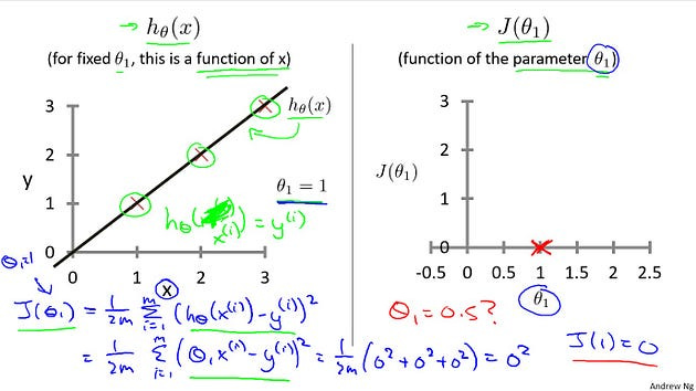
Let’s plot these functions and try to understand them both better. Let’s start with the hypothesis. On the left, let’s say here’s my training set with three points at (1, 1), (2, 2), and (3, 3).
Let’s pick a value theta one, so when theta one equals one, and if that’s my choice for theta one, then my hypothesis is going to look like this straight line over here. And I’m gonna point out, when I’m plotting my hypothesis function. X-axis, my horizontal axis is labeled X, is labeled you know, size of the house over here. Now, of temporary, set theta one equals one, what I want to do is figure out what is j of theta one, when theta one equals one. So let’s go ahead and compute what the cost function has for. You’ll devalue one. Well, as usual, my cost function is defined as follows, right? Some from, some of ’em are training sets of this usual squared error term. And, this is therefore equal to. And this. Of theta one x I minus y I and if you simplify this turns out to be. That. Zero Squared to zero squared to zero squared which is of course, just equal to zero. Now, inside the cost function. It turns out each of these terms here is equal to zero. Because for the specific training set I have or my 3 training examples are (1, 1), (2, 2), (3,3). If theta one is equal to one. Then h of x. H of x i. Is equal to y I exactly, let me write this better. Right? And so, h of x minus y, each of these terms is equal to zero, which is why I find that j of one is equal to zero. So, we now know that j of one Is equal to zero.Let’s plot that. What I’m gonna do on the right is plot my cost function j. And notice, because my cost function is a function of my parameter theta one, when I plot my cost function, the horizontal axis is now labeled with theta one. So I have j of one zero zero so let’s go ahead and plot that. End up with. An X over there.
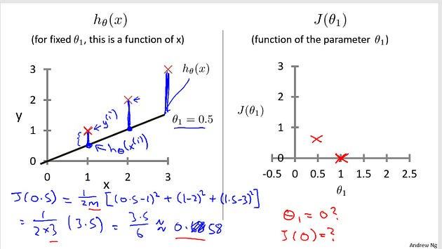
Now lets look at some other examples. Theta-1 can take on a range of different values. Right? So theta-1 can take on the negative values, zero, positive values. So what if theta-1 is equal to 0.5. What happens then? Let’s go ahead and plot that. I’m now going to set theta-1 equals 0.5, and in that case my hypothesis now looks like this. As a line with slope equals to 0.5, and, lets compute J, of 0.5. So that is going to be one over 2M of, my usual cost function.It turns out that the cost function is going to be the sum of square values of the height of this line. Plus the sum of square of the height of that line, plus the sum of square of the height of that line, right? ?Cause just this vertical distance, that’s the difference between, you know, Y. I. and the predicted value, H of XI, right? So the first example is going to be 0.5 minus one squared. Because my hypothesis predicted 0.5. Whereas, the actual value was one. For my second example, I get, one minus two squared, because my hypothesis predicted one, but the actual housing price was two. And then finally, plus. 1.5 minus three squared. And so that’s equal to one over two times three. Because, M when trading set size, right, have three training examples. In that, that’s times simplifying for the parentheses it’s 3.5. So that’s 3.5 over six which is about 0.68.So now we know that j of 0.5 is about 0.68. Lets go and plot that. Oh excuse me, math error, it’s actually 0.58. So we plot that which is maybe about over there.
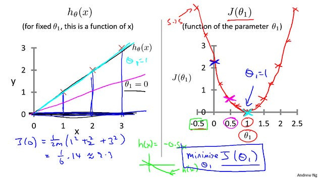
Okay? Now, let’s do one more. How about if theta one is equal to zero, what is J of zero equal to? It turns out that if theta one is equal to zero, then H of X is just equal to, you know, this flat line, right, that just goes horizontally like this. And so, measuring the errors. We have that J of zero is equal to one over two M, times one squared plus two squared plus three squared, which is, One six times fourteen which is about 2.3. So let’s go ahead and plot as well. So it ends up with a value around 2.3
and of course, we can keep on doing this for other values of theta one. It turns out that you can have you know negative values of theta one as well so if theta one is negative then h of x would be equal to say minus 0.5 times x then theta one is minus 0.5 and so that corresponds to a hypothesis with a slope of negative 0.5. And you can actually keep on computing these errors. This turns out to be, you know, for 0.5, it turns out to have really high error. It works out to be something, like, 5.25.
And so on, and the different values of theta one, you can compute these things, right? And it turns out that you, your computed range of values, you get something like that. And by computing the range of values, you can actually slowly create out. What does function J of Theta say and that’s what J of Theta is.
To recap, for each value of theta one, right? Each value of theta one corresponds to a different hypothesis, or to a different straight line fit on the left. And for each value of theta one, we could then derive a different value of j of theta one. And for example, you know, theta one=1, corresponded to this straight line straight through the data. Whereas theta one=0.5. And this point shown in magenta corresponded to maybe that line, and theta one=zero which is shown in blue corresponds to this horizontal line. Right, so for each value of theta one we wound up with a different value of J of theta one and we could then use this to trace out this plot on the right.
Now you remember, the optimization objective for our learning algorithm is we want to choose the value of theta one. That minimizes J of theta one. Right? This was our objective function for the linear regression.
Well, looking at this curve, the value that minimizes j of theta one is, you know, theta one equals to one. And low and behold, that is indeed the best possible straight line fit through our data, by setting theta one equals one. And just, for this particular training set, we actually end up fitting it perfectly. And that’s why minimizing j of theta one corresponds to finding a straight line that fits the data well.

So, to wrap up. In this tutorial, we looked up some plots. To understand the cost function. To do so, we simplify the algorithm. So that it only had one parameter theta one. And we set the parameter theta zero to be only zero.
Please Subscribe 👏Course teach for Indepth study of Supervised Learning with Sklearn
🚀 Elevate Your Data Skills with Coursesteach! 🚀
Ready to dive into Python, Machine Learning, Data Science, Statistics, Linear Algebra, Computer Vision, and Research? Coursesteach has you covered!
🔍 Python, 🤖 ML, 📊 Stats, ➕ Linear Algebra, 👁️🗨️ Computer Vision, 🔬 Research — all in one place!
Enroll now for top-tier content and kickstart your data journey!
Supervised learning with scikit-learn
🔍 Explore cutting-edge tools and Python libraries, access insightful slides and source code, and tap into a wealth of free online courses from top universities and organizations. Connect with like-minded individuals on Reddit, Facebook, and beyond, and stay updated with our YouTube channel and GitHub repository. Don’t wait — enroll now and unleash your ML with Sklearn potential!”
Stay tuned for our upcoming articles because we reach end to end ,where we will explore specific topics related to Supervised learning with sklearn in more detail!
Remember, learning is a continuous process. So keep learning and keep creating and Sharing with others!💻✌️
We offer following serveries:
We offer the following options:
Enroll in my ML Libraries course: You can sign up for the course at this link. The course is designed in a blog-style format and progresses from basic to advanced levels.
Access free resources: I will provide you with learning materials, and you can begin studying independently. You are also welcome to contribute to our community — this option is completely free.
Online tutoring: If you’d prefer personalized guidance, I offer online tutoring sessions, covering everything from basic to advanced topics. please contact:mushtaqmsit@gmail.com
Contribution: We would love your help in making coursesteach community even better! If you want to contribute in some courses , or if you have any suggestions for improvement in any coursesteach content, feel free to contact and follow.
Together, let’s make this the best AI learning Community! 🚀
Together, let’s make this the best AI learning Community! 🚀
References
1- Machine Learning (Andrew)
2- Google Bard
3-Cost Function — Intuition1(Video)