


Gradient Descent for Multiple Variables: A Complete Guide with Python Implementation
Machine learning (Part 17)

📚Chapter: 4 -Linear Regression with Multiple Variable
If you want to read more articles about Machine Learning n, don’t forget to stay tuned :) click here.
Description
In the previous Tutorial, we talked about the form of the hypothesis for linear regression with multiple features or with multiple variables. In this Tutorial, let’s talk about how to fit the parameters of that hypothesis. In particular let’s talk about how to use gradient descent for linear regression with multiple features. In the realm of machine learning, the journey from raw data to predictive models involves a multitude of algorithms and techniques. Among these, gradient descent stands out as a fundamental optimization algorithm, especially when dealing with models that have multiple variables. This blog post will delve into the intricacies of gradient descent for multiple variables, shedding light on its significance and the mechanics that drive it.
Section 1- Understanding Gradient Descent :
At its core, gradient descent is an optimization algorithm used to minimize a function iteratively. Whether we are dealing with linear regression, neural networks, or any other model with multiple parameters, the primary goal is to find the set of parameters that minimizes a cost function, also known as the loss function.
For a model with multiple variables, the cost function becomes a multidimensional surface, and the challenge is to find the global minimum efficiently. Gradient descent addresses this challenge by iteratively adjusting the model parameters in the direction opposite to the gradient of the cost function.
Section 2- Mathematics Behind Gradient Descent for Multiple Variables (Dr Andrew)

To quickly summarize our notation, this is our formal hypothesis in multivariable linear regression where we’ve adopted the convention that x0=1. The parameters of this model are theta0 through theta n, but instead of thinking of this as n separate parameters, which is valid, I’m instead going to think of the parameters as theta where theta here is a n+1-dimensional vector. So I’m just going to think of the parameters of this model as itself being a vector. Our cost function is J of theta0 through theta n which is given by this usual sum of square of error term. But again instead of thinking of J as a function of these n+1 numbers, I’m going to more commonly write J as just a function of the parameter vector theta so that theta here is a vector.
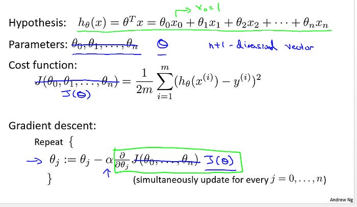
Here’s what gradient descent looks like. We’re going to repeatedly update each parameter theta j according to theta j minus alpha times this derivative term. And once again we just write this as J of theta, so theta j is updated as theta j minus the learning rate alpha times the derivative, a partial derivative of the cost function with respect to the parameter theta j. Let’s see what this looks like when we implement gradient descent and, in particular, let’s go see what that partial derivative term looks like. Here’s what we have for gradient descent for the case of when we had N=1 feature. We had two separate update rules for the parameters theta0 and theta1, and hopefully these look familiar to you. And this term here was of course the partial derivative of the cost function with respect to the parameter of theta0, and similarly we had a different update rule for the parameter theta1. There’s one little difference which is that when we previously had only one feature, we would call that feature x(i) but now in our new notation we would of course call this x(i)<u>1 to denote our one feature.</u> So that was for when we had only one feature. Let’s look at the new algorithm for we have more than one feature, where the number of features n may be much larger than one. We get this update rule for gradient descent and, maybe for those of you that know calculus, if you take the definition of the cost function and take the partial derivative of the cost function J with respect to the parameter theta j, you’ll find that that partial derivative is exactly that term that I’ve drawn the blue box around. And if you implement this you will get a working implementation of gradient descent for multivariate linear regression. The last thing I want to do on this slide is give you a sense of why these new and old algorithms are sort of the same thing or why they’re both similar algorithms or why they’re both gradient descent algorithms. Let’s consider a case where we have two features or maybe more than two features, so we have three update rules for the parameters theta0, theta1, theta2 and maybe other values of theta as well. If you look at the update rule for theta0, what you find is that this update rule here is the same as the update rule that we had previously for the case of n = 1. And the reason that they are equivalent is, of course, because in our notational convention we had this x(i)<u>0 = 1 convention, which is</u> why these two term that I’ve drawn the magenta boxes around are equivalent. Similarly, if you look the update rule for theta1, you find that this term here is equivalent to the term we previously had, or the equation or the update rule we previously had for theta1, where of course we’re just using this new notation x(i)<u>1 to denote</u> our first feature, and now that we have more than one feature we can have similar update rules for the other parameters like theta2 and so on. There’s a lot going on on this slide so I definitely encourage you if you need to to pause the Tutorial and look at all the math on this slide slowly to make sure you understand everything that’s going on here. But if you implement the algorithm written up here then you have a working implementation of linear regression with multiple features.
Section 3- Challenges and Techniques:
Optimizing a cost function with multiple variables presents unique challenges. The choice of the learning rate is critical, as a too small rate can result in slow convergence, while a too large rate may cause overshooting and divergence.
Additionally, the cost function’s shape can influence the algorithm’s performance. If the cost function has narrow, steep valleys, gradient descent might oscillate or converge slowly. Techniques like feature scaling, regularization, and advanced optimization algorithms (e.g., Adam or RMSprop) can mitigate these challenges.
Section 4- Vectorized Implementation:
Efficiency is paramount in machine learning, and vectorized implementations can significantly speed up the optimization process. Vectorization allows simultaneous operations on entire matrices, leveraging hardware acceleration for faster computations.
Section 5- Python code for gradient descent for multiple variables (multiple features).
import numpy as npdef normalize_features(X):
"""
Normalize features to have zero mean and unit variance.
"""
mean = np.mean(X, axis=0)
std = np.std(X, axis=0)
X_normalized = (X - mean) / std
return X_normalized, mean, stddef add_bias_feature(X):
"""
Add a bias feature (constant 1) to the input matrix.
"""
return np.column_stack((np.ones(len(X)), X))def compute_cost(X, y, theta):
"""
Compute the cost function for linear regression.
"""
m = len(y)
h = X.dot(theta)
cost = (1 / (2 * m)) * np.sum((h - y) ** 2)
return costdef gradient_descent(X, y, theta, alpha, num_iterations):
"""
Perform gradient descent to minimize the cost function.
"""
m = len(y)
cost_history = []
for _ in range(num_iterations):
h = X.dot(theta)
error = h - y
gradient = (1 / m) * X.T.dot(error)
theta = theta - alpha * gradient
cost = compute_cost(X, y, theta)
cost_history.append(cost)
return theta, cost_history# Sample data generation
np.random.seed(42)
X = 2 * np.random.rand(100, 3) # 100 samples with 3 features
y = 4 + X.dot(np.array([3, 1.5, 2])) + np.random.randn(100)
# Normalize features and add bias feature
X_normalized, mean, std = normalize_features(X)
X_bias = add_bias_feature(X_normalized)
# Initial parameters
theta_initial = np.zeros(X_bias.shape[1])
# Hyperparameters
alpha = 0.01
num_iterations = 1000
# Run gradient descent
theta_final, cost_history = gradient_descent(X_bias, y, theta_initial, alpha, num_iterations)
# Print the final parameters and cost
print("Final Parameters:", theta_final)
print("Final Cost:", cost_history[-1])# Plot the cost history
import matplotlib.pyplot as plt
plt.plot(cost_history)
plt.xlabel('Iteration')
plt.ylabel('Cost')
plt.title('Cost History during Gradient Descent')
plt.show()Conclusion:
Gradient descent for multiple variables is a cornerstone of machine learning optimization. Understanding its mechanics and nuances is crucial for practitioners aiming to build robust and efficient models. As you embark on your machine learning journey, keep in mind that gradient descent is a powerful tool that, when wielded skillfully, can unlock the true potential of your models in the vast landscape of data science.
Please Subscribe 👏Course teach for Indepth study of Machine Learning
🚀 Elevate Your Data Skills with Coursesteach! 🚀
Ready to dive into Python, Machine Learning, Data Science, Statistics, Linear Algebra, Computer Vision, and Research? Coursesteach has you covered!
🔍 Python, 🤖 ML, 📊 Stats, ➕ Linear Algebra, 👁️🗨️ Computer Vision, 🔬 Research — all in one place!
Don’t Miss Out on This Exclusive Opportunity to Enhance Your Skill Set! Enroll Today 🌟 at

Understanding of Machine Learning Course!
Artificial Intelligence Career Advice Course
Stay tuned for our upcoming articles because we research end to end , where we will explore specific topics related to Machine Learning in more detail!
🔍 Explore Tools, Python libraries for ML, Slides, Source Code, Free Machine Learning Courses from Top Universities and More!
Remember, learning is a continuous process. So keep learning and keep creating and Sharing with others!💻✌️
Note:if you are a Machine Learning export and have some good suggestions to improve this blog to share, you write comments and contribute.
if you need more update about Machine Learning and want to contribute then following and enroll in following
👉Course: Machine Learning (ML)
We offer following serveries:
We offer the following options:
Enroll in my ML course: You can sign up for the course at this link. The course is designed in a blog-style format and progresses from basic to advanced levels.
Access free resources: I will provide you with learning materials, and you can begin studying independently. You are also welcome to contribute to our community — this option is completely free.
Online tutoring: If you’d prefer personalized guidance, I offer online tutoring sessions, covering everything from basic to advanced topics. please contact:mushtaqmsit@gmail.com
Contribution: We would love your help in making coursesteach community even better! If you want to contribute in some courses , or if you have any suggestions for improvement in any coursesteach content, feel free to contact and follow.
Together, let’s make this the best AI learning Community! 🚀
References
1- Machine Learning — Andrew