Gradient Descent Explained: A Beginner’s Guide to Optimizing Machine Learning Models

ML(Part 7)

📚Chapter:2-Regression

If you want to read more articles about Supervise Learning with Sklearn, don’t forget to stay tuned :) click here.

Description:

In this blog post, we will delve into the concept of gradient descent, a widely used optimization algorithm in the field of machine learning and data science. By understanding how gradient descent works and its various variants, you will gain valuable insights into how it can be applied to solve complex optimization problems. Whether you are a beginner or an experienced practitioner, this comprehensive guide will equip you with the knowledge needed to effectively leverage gradient descent in your projects. In this blog, I want to tell you about an algorithm called gradient descent for minimizing the cost function J.

Section 1: Introduction to Optimization

Optimization lies at the heart of numerous computational problems, ranging from finding the optimal parameters for a machine learning model to minimizing the cost function of a neural network and linear regression. Gradient descent is a powerful optimization algorithm that iteratively updates the parameters of a model to minimize a given objective function. Let’s explore how gradient descent achieves this objective.

Section 2: The Intuition Behind Gradient Descent

To comprehend gradient descent, it is crucial to grasp the intuition behind it. Imagine standing on a mountain and trying to find the fastest route downhill. You would take small steps in the steepest direction downwards until you reach the bottom. Similarly, gradient descent operates by iteratively adjusting the parameters of a model in the direction of the steepest descent to reach the global minimum of the objective function.

Suppose that John is on the top of a mountain, and his goal is to reach the bottom field, but John is blind and cannot see the bottom line. How will he solve this problem [2] To solve this problem, he will take small steps around and move towards the higher incline direction, applying these steps iteratively by moving one step at a time until he finally reaches the base of the mountain [2] Gradient descent performs in the same way as mentioned in the example. Its primary purpose is to reach the lowest point of the mountain [2].

Gradient Descent is like a Blind man looking for the clearest route to the bottom of a cost function — think of the cost function as a mountain. The aim is to find the parameter values of the model that will reduce the cost as much as possible.

A gradient simply measures the change in all weights with regard to the change in error. This means that the lower the gradient, the flatter the slope, and the slower a model learns. The opposite is also true: the higher the gradient, the steeper the slope, and the faster a model will learn.

Section 3: The Mathematics of Gradient Descent

To implement gradient descent, we need to understand the mathematical foundations. At its core, gradient descent computes the gradient of the objective function with respect to the parameters. The gradient is a vector that points in the direction of the steepest ascent. By taking steps in the opposite direction of the gradient, we descend towards the minimum. The size of each step is determined by the learning rate, which balances convergence speed and stability.

Section 4: Definition of Gradient Descent

It turns out gradient descent is a more general algorithm and is used not only in linear regression. It’s actually used all over the place in machine learning [1] Gradient descent is one of the most common machine learning algorithms used in neural networks, data science, optimization, and machine learning tasks. The gradient descent algorithm and its variants can be found in almost every machine-learning model [2]. The Gradient Descent algorithm is the essence of many machine learning algorithms, especially in neural networks as well as in any prediction task. This algorithm is used for many AI applications, from face recognition to other computer vision products, for different predictions, both for predictions of the continuous target (i.e. regression, e.g. price) or categorical one (i.e. probability for some outcome) [3].In the gradient descent algorithm, the parts are the gradient, which is, let’s say simply the relationship of change between two parameters and descent, some point in this relation which minimizes some desired parameter. But what do we want to minimize? The Cost Function. What is the cost function?

Def: Now we can define gradient descent. This optimization algorithm finds the values of a function’s parameters that minimize the cost function. The cost function is simply the method of evaluation chosen to communicate the performance of an algorithm

Def: Gradient descent is a popular optimization method of tuning the parameters in a machine learning model. Its goal is to apply optimization to find the least or minimal error value. It is mostly used to update the parameters of the model — in this case, parameters refer to coefficients in regression and weights in a neural network [2] . A gradient is a vector-valued function that describes the slope of the tangent of a function’s graph, pointing to the direction of the most significant rate of increase of the function. It is a derivative that shows the incline or the slope of a cost function [2] Gradient descent is an efficient optimization algorithm that attempts to find a local or global minimum of the cost function [2] Suppose we have a function with n variables, then the gradient is the length-n vector that defines the direction in which the cost is increasing most rapidly. So in gradient descent, we follow the negative of the gradient to the point where the cost is a minimum. In machine learning, the cost function is a function to which we are applying the gradient descent algorithm[2]

Section 5: Global minima and local minima

A local minimum is a point where our function is lower than all neighboring points. It is not possible to decrease the value of the cost function by making infinitesimal steps. [2] A global minimum is a point that obtains the absolute lowest value of our function, but global minima are difficult to compute in practice [2].

Local minima refer to points in an optimization problem where the objective function has a lower value compared to its neighboring points. In other words, it is a solution that appears to be optimal within a specific region of the search space. However, it may not necessarily be the best solution overall. In mathematical terms, a point x is considered a local minimum if there exists a neighborhood around x such that f(x*) ≤ f(x) for all x within that neighborhood. It is important to note that this definition implies that the objective function can have multiple local minima within different regions of the search space.

Global minima, on the other hand, represent the absolute best solution across the entire search space. It is the point where the objective function has the lowest value compared to all other points in the search space. Finding the global minimum is crucial as it guarantees the optimal solution for the optimization problem.

Formally, a point x is considered a global minimum if f(x) ≤ f(x) for all x within the search space. Unlike local minima, there can only be one global minimum for a given optimization problem.

To better differentiate between local and global minima, let’s consider an analogy. Imagine you are hiking in a mountainous region with several peaks. Each peak represents a local minimum, while the highest peak among them represents the global minimum. While you may reach the top of a local peak, it does not guarantee that you have reached the highest peak in the entire region.

Similarly, in optimization problems, local minima may seem optimal within a specific region, but they might not represent the best solution overall. The global minimum, on the other hand, ensures that we have found the most optimal solution across the entire search space.

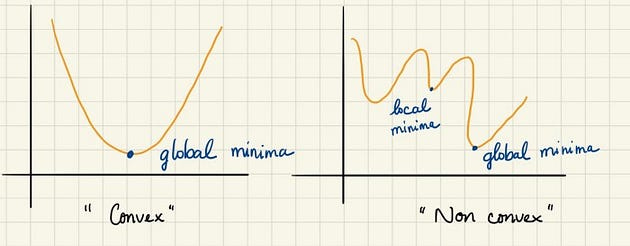
Section 6: Convex and Nonconvex

A function is said to be convex if, for any two points in its domain, the line segment connecting them lies entirely above the graph of the function. In simpler terms, a function is convex if it curves upward or remains flat, never dipping below its graph. Convex functions possess several important properties that make them particularly useful in mathematical modeling and optimization. Here are some key properties of convex functions: Global Minimum: Convex functions have a unique global minimum, which means that any local minimum is also the global minimum.

While convex functions have well-defined properties and provide convenient solutions to optimization problems, non-convex functions present more complex challenges. A function is considered non-convex if it fails to satisfy the condition of convexity mentioned earlier. In other words, a non-convex function can have regions where its graph dips below the line segment connecting any two points in its domain.

Here are some notable difficulties associated with non-convex functions: Multiple Local Minima: Unlike convex functions that have a unique global minimum, non-convex functions may have multiple local minima. This makes it difficult to find the optimal solution efficiently.

When a cost function is non-convex it has a high chance of finding local minima rather than the global minimum which is usually undesirable in machine learning models from an optimization standpoint. A Convex function has one minimum a nice property as an optimization algorithm won’t get stuck in a local minimum that is not a global minimum A non-convex function is wavy and has some valleys (local minima) that are not as deep as the overall deepest valley (global minimum) Optimization algorithms can get stuck in the local minima

Section 7: Derivative or Slop

Directional Derivatives

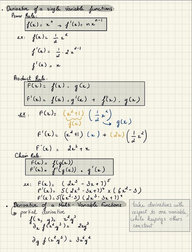
Machine learning uses derivatives in optimization problems. Derivatives are used to decide whether to increase or decrease the weights to increase or decrease an objective function. If we can compute the derivative of a function, we know in which direction to proceed to minimize it.[2] For a function z=f(x,y), the partial derivative with respect to x gives the rate of change of f in the x-direction and the partial derivative with respect to y gives the rate of change of f in the y-direction. How do we compute the rate of change of f in an arbitrary direction? The rate of change of a function of several variables in the direction u is called the directional derivative in the direction u. Here u is assumed to be a unit vector. Assuming w=f(x,y,z) and u=<u_1,u_2,u_3>

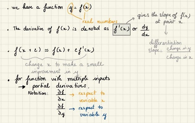
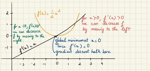
Suppose we have a function y = f(x) . The derivative f’(x) gives the slope of f(x) at point x. It specifies how to scale a small change in the input to obtain the corresponding change in the output. Let’s say, f(x) = 1/2 x²

Section 8: How Gradient Descent works

I’m going to talk about gradient descent for minimizing some arbitrary function J. And then in later tutoiral, we’ll take that algorithm and apply it specifically to the cost function J that we had to find for linear regression. So here’s the problem setup. We’re going to see that we have some function J of (theta0, theta1). Maybe it’s a cost function from linear regression. Maybe it’s some other function we want to minimize. And we want to come up with an algorithm for minimizing that as a function of J of (theta0, theta1).

Machine Learning — Andrew

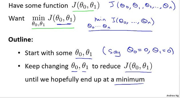
Just as an aside, it turns out that gradient descent actually applies to more general functions. So imagine if you have a function that’s a function of J of (theta0, theta1, theta2, up to some theta n). And you want to minimize over (theta0 up to theta n) of this J of (theta0 up to theta n). It turns out gradient descent is an algorithm for solving this more general problem, but for the sake of brevity, for the sake of your succinctness of notation, I’m just going to present only two parameters throughout the rest of this tutorial.

Here’s the idea for gradient descent. What we’re going to do is we’re going to start off with some initial guesses for theta0 and theta1. Doesn’t really matter what they are, but a common choice would be if we set theta0 to 0, and set theta1 to 0. Just initialize them to 0.

What we’re going to do in gradient descent is we’ll keep changing theta0 and theta1 a little bit to try to reduce J of (theta0, theta1) until hopefully, we wind up at a minimum or maybe a local minimum.

Machine Learning — Andrew

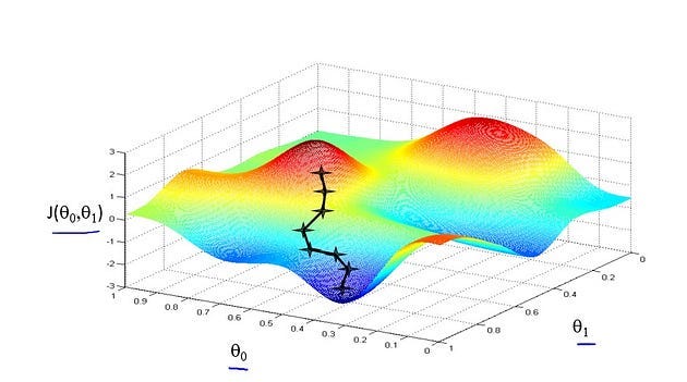
So, let’s see pictures of what gradient descent does. Let’s say I try to minimize this function. So notice the axes. This is, (theta0, theta1) on the horizontal axes, and J is a vertical axis. And so the height of the surface shows J, and we want to minimize this function. So, we’re going to start off with (theta0, theta1) at some point. So imagine picking some value for (theta0, theta1), and that corresponds to starting at some point on the surface of this function. Okay? So whatever value of (theta0, theta1) gives you some point here. I did initialize them to 0, but sometimes you initialize it to other values as well. Now. I want us to imagine that this figure shows a hill. Imagine this is like a landscape of some grassy park with two hills like so. And I want you to imagine that you are physically standing at that point on the hill on this little red hill in your park. In gradient descent, what we’re going to do is spin 360 degrees around and just look all around us and ask, “If I were to take a little baby step in some direction, and I want to go downhill as quickly as possible, what direction do I take that little baby step in if I want to go down, if I sort of want to physically walk down this hill as rapidly as possible?” Turns out that if we’re standing at that point on the hill, you look all around, you find that the best direction to take a little step downhill is roughly that direction. Okay. And now you’re at this new point on your hill. You’re going to, again, look all around, and then say, “What direction should I step in order to take a little baby step downhill?”

Machine Learning — Andrew

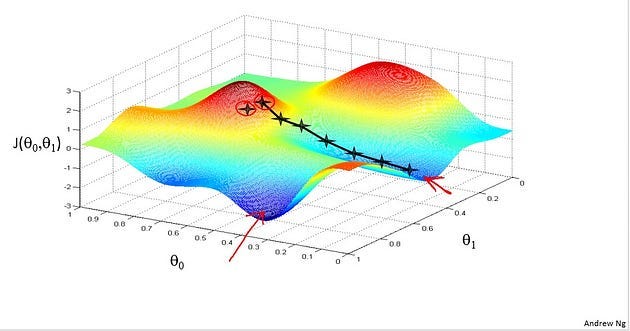
And if you do that and take another step, you take a step in that direction, and then you keep going. You know, from this new point, you look around, decide what direction will take you downhill most quickly, take another step, another step, and so on, until you converge to this, Local minimum down here. Further descent has an interesting property. This first time we ran gradient descent, we were starting at this point over here, right? Started at that point over here. Now imagine, we initialize gradient descent just a couple of steps to the right. Imagine we initialized gradient descent with that point on the upper right. If you were to repeat this process, and stop at the point, and look all around. Take a little step in the direction of the steepest descent. You would do that. Then look around, take another step, and so on. And if you start it just a couple steps to the right, the gradient descent will have taken you to this second local optimum over on the right.

So if you had started at this first point, you would have wound up at this local optimum. But if you started just a little bit, a slightly different location, you would have wound up at a very different local optimum. And this is a property of gradient descent that we’ll say a little bit more about later. So, that’s the intuition in pictures. Let’s look at the map. This is the definition of the gradient descent algorithm. We’re going to just repeatedly do this. On to convergence. We’re going to update my parameter theta j by, you know, taking theta j and subtracting from it alpha times this term over here.

Machine Learning — Andrew

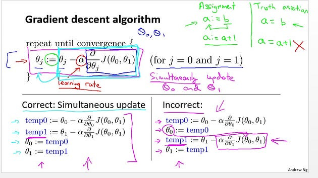
So, let’s see. There are a lot of details in this equation, so let me unpack some of it. First, this notation here, colon equals. We’re going to use:= to denote assignment, so it’s the assignment operator. So concretely, if I write A: =B, what this means in a computer, this means take the value in B and use it to overwrite whatever the value of A. So this means we will set A to be equal to the value of B.

Okay, it’s assignment. I can also do A:=A+1. This means take A and increase its value by one.

Whereas in contrast, if I use the equals sign and I write A=B, then this is a truth assertion. So if I write A=B, then I’m asserting that the value of A equals to the value of B.

So the left hand side, that’s a computer operation, where you set the value of A to be a value. The right hand side, this is asserting, I’m just making a claim that the values of A and B are the same. And so, whereas I can write A: =A+1, that means increment A by 1. Hopefully, I won’t ever write A=A+1. Because that’s just wrong. A and A+1 can never be equal to the same values. So that’s the first part of the definition.

Alpha

This alpha here is a number that is called the learning rate. And what alpha does is, it basically control how big a step we take downhill with gradient descent. So if alpha is very large, then that corresponds to a very aggressive gradient descent procedure, where we’re trying to take huge steps downhill. And if alpha is very small, then we’re taking little, little baby steps downhill. And, I’ll come back and say more about this later. About how to set alpha and so on. And finally, this term here. That’s the derivative term, I don’t want to talk about it right now, but I will derive this derivative term and tell you exactly what this is based on.

Now there’s one more subtlety about gradient descent which is, in gradient descent, we’re going to update theta0 and theta1. So this update takes place where j=0, and j=1. So you’re going to update j, theta0, and update theta1.

Simultaneously update

And the subtlety of how you implement gradient descent is, for this expression, for this update equation, you want to simultaneously update theta0 and theta1. What I mean by that is that in this equation, we’re going to update theta0:=theta0 — something, and update theta1:=theta1 — something.
And the way to implement this is, you should compute the right-hand side. Compute that thing for both theta0 and theta1, and then simultaneously at
the same time update theta0 andtheta1.

So let me say what I mean by that. This is a correct implementation of gradient descent meaning simultaneous updates. I’m going to set temp0 equals that, set temp1 equals that. So basically compute the right hand sides. And then having computed the right hand sides and stored them together in temp0 and temp1, I’m going to update theta0 and theta1 simultaneously because that’s the correct implementation. In contrast, here’s an incorrect implementation that does not do a simultaneous update.

So in this incorrect implementation, we compute temp0, and then we update theta0 and then we compute temp1. Then we update temp1. And the difference between the right hand side and the left hand side implementations is that if we look down here, you look at this step, if by this time you’ve already updated theta0 then you would be using the new value of theta0 to compute this derivative term and so this gives you a
different value of temp1 than the left hand side, because you’ve now plugged in the new value of theta0 into this equation. And so this on right hand side is not a correct implementation of gradient descent. So I don’t want to say why you need to do the simultaneous updates, it turns out that the way gradient descent is usually implemented, we’ll say more about it later, it actually turns out to be more natural to implement the simultaneous update. And when people talk about gradient descent, they always mean simultaneous update. If you implement the non-simultaneous update, it turns out it will probably work anyway, but this algorithm on the right is not what people people refer to as gradient descent and this is some other algorithm with different properties. And for various reasons, this can behave in slightly stranger ways. And what you should do is to really implement the simultaneous update of gradient descent. So, that’s the outline of the gradient descent algorithm.

Section 8: Steps of Gradient Descent

Gradient descent finds these optimal parameters by determining the local minimum of a differentiable function through an iterative process. The following equation describes gradient descent:

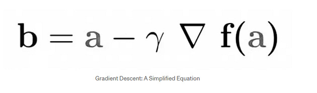
In this equation:

1. b describes the next iteration

2. a describes the current iteration: gradient descent starts with random values of a and b and then keeps updating these values based on the first-order partial derivatives

3. The minus sign describes the minimization aspect of gradient descent

4. 𝛾 describes the learning rate, which will be discussed more in-depth further on in the article

5. The gradient term describes the direction of the steepest descent

Section 9: Batch Gradient Descent

Batch gradient descent is the simplest variant of gradient descent. It calculates the gradient using the entire training dataset at each iteration. While this approach guarantees convergence to the global minimum, it can be computationally expensive for large datasets. Nonetheless, batch gradient descent serves as a fundamental building block for understanding more advanced variants.

Section 10: Stochastic Gradient Descent

Stochastic gradient descent (SGD) addresses the computational inefficiency of batch gradient descent by randomly selecting a single data point or a small batch of data points to compute the gradient. This stochastic nature introduces variability but allows for faster convergence. SGD is particularly useful when dealing with large datasets or online learning scenarios where new data arrives continuously.

Section 11: Mini-Batch Gradient Descent

Mini-batch gradient descent lies in between batch gradient descent and stochastic gradient descent. It computes the gradient using a small randomly selected subset of the training data at each iteration. This approach strikes a balance between computational efficiency and convergence speed, making it a popular choice in practice.

Section 12: Gradient Descent Variants

While batch, stochastic, and mini-batch gradient descent are commonly used variants, several other variations exist. Some notable examples include momentum-based methods like Nesterov accelerated gradient (NAG), which helps accelerate convergence by incorporating information from previous iterations. Additionally, AdaGrad and RMSprop are adaptive learning rate methods that adjust the learning rate for each parameter independently based on historical gradients.

Section 13: Practical Considerations and Challenges

Implementing gradient descent effectively requires considering various practical aspects. Choosing an appropriate learning rate, initializing model parameters correctly, and handling features with different scales are some common challenges. Regularization techniques such as L1 or L2 regularization can also be employed to prevent overfitting. Understanding these practical considerations is crucial for obtaining reliable and robust results.

Section 14: Applications in Machine Learning and Data Science

Gradient descent finds extensive applications in diverse areas of machine learning and data science. It is an essential component in training deep neural networks, optimizing regression models, and fine-tuning hyperparameters. By grasping the underlying principles of gradient descent, you will be equipped to tackle a wide range of optimization problems that arise in real-world scenarios.

Section 15: Conclusion

Gradient descent is a fundamental optimization algorithm that plays a pivotal role in various domains, especially machine learning and data science. By understanding its intuition, mathematics, variants, and practical considerations, you can leverage gradient descent to optimize models effectively. Armed with this knowledge, you are now better equipped to tackle complex optimization problems and unlock new possibilities in your projects.

Please Subscribe 👏Course teach for Indepth study of Supervised Learning with Sklearn

🚀 Elevate Your Data Skills with Coursesteach! 🚀

Ready to dive into Python, Machine Learning, Data Science, Statistics, Linear Algebra, Computer Vision, and Research? Coursesteach has you covered!

🔍 Python, 🤖 ML, 📊 Stats, ➕ Linear Algebra, 👁️‍🗨️ Computer Vision, 🔬 Research — all in one place!

Don’t Miss Out on This Exclusive Opportunity to Enhance Your Skill Set! Enroll Today 🌟 at

Artificial Intelligence Career Advice Course

Stay tuned for our upcoming articles because we research end to end , where we will explore specific topics related to Machine Learning in more detail!

🔍 Explore Tools, Python libraries for ML, Slides, Source Code, Free Machine Learning Courses from Top Universities and More!

Remember, learning is a continuous process. So keep learning and keep creating and Sharing with others!💻✌️

Note:if you are a Machine Learning export and have some good suggestions to improve this blog to share, you write comments and contribute.

if you need more update about Machine Learning and want to contribute then following and enroll in following

👉Course: Machine Learning (ML)

👉📚GitHub Repository

👉 📝Notebook

We offer following serveries:
We offer the following options:

1. Enroll in my ML course: You can sign up for the course at this link. The course is designed in a blog-style format and progresses from basic to advanced levels.

2. Access free resources: I will provide you with learning materials, and you can begin studying independently. You are also welcome to contribute to our community — this option is completely free.

3. Online tutoring: If you’d prefer personalized guidance, I offer online tutoring sessions, covering everything from basic to advanced topics. please contact:mushtaqmsit@gmail.com

Contribution: We would love your help in making coursesteach community even better! If you want to contribute in some courses , or if you have any suggestions for improvement in any coursesteach content, feel free to contact and follow.

Together, let’s make this the best AI learning Community! 🚀

👉WhatsApp

👉 Facebook

👉Github

👉LinkedIn

👉Youtube

👉Twitter

Source

1- Machine Learning — Andrew

2-Gradient Descent for Machine Learning (ML) 101 with Python Tutorial

3- The Magic of Machine Learning: Gradient Descent Explained Simply but With All Math

4-Gradient Descent: Explained!