Essential Image Processing Techniques for Machine Learning & AI

Project 1

Introduction

In the realm of machine learning and computer vision, the quality of your model’s output heavily relies on the quality of the input data. Image data preprocessing is a crucial step that can significantly influence the performance of your model. When given a dataset, the preprocessing can have various steps depending on a) what type of data you’re looking at (text, images, time series, …) b) what models you want to train

This blog will walk you through the essentials of image data preprocessing in Python, using popular libraries like OpenCV, PIL, and TensorFlow.

Sections

What is image Preprocessing
Tools and Libraries
Image Preprocessing steps
Conclusion

Section 1- Basics of Image Processing

What is preprocessing?

Def: Preprocessing describes the process of cleaning and converting a ‘raw’ (i.e. unprocessed) dataset into a clean dataset.

Def: Image preprocessing is the process of manipulating raw image data into a usable and meaningful format. It allows you to eliminate unwanted distortions and enhance specific qualities essential for computer vision applications.

Def: Image processing involves manipulating and analyzing digital images to enhance their quality or extract meaningful information.

Why Image Data Preprocessing?

Before feeding images into a machine learning model, preprocessing is necessary for several reasons:

1- Normalization: Ensures that pixel values are within a specific range.

2- Resizing: Standardizes the input size for uniformity.

3- Augmentation: Increases the diversity of the training data without actually collecting new data.

4- Noise Reduction: Removes unwanted artifacts that can distort the image.

Section 2- Tools and Libraries

Several libraries exist that make it easier to preprocess images. For example, you can use scikit-image, OpenCV **or **Pillow. Each library has different functionalities, pros and cons. In this notebook we will stick to scikit-image.

Tools and Libraries

OpenCV
PIL (Pillow)
TensorFlow
scikit-image
NumPy
Matplotlib
‘

Python offers several libraries to handle image data preprocessing:

1- OpenCV (Open-Source Computer Vision Library): OpenCV is one of the most popular libraries for computer vision and image processing. It provides a wide range of functions for image and video analysis, including reading and writing images, image transformations, feature detection, and much more.

2- PIL (Pillow): A Python Imaging Library that adds image processing capabilities.A fork of the Python Imaging Library (PIL) offering simple image processing capabilities

3- TensorFlow: An end-to-end open-source platform for machine learning that includes preprocessing utilities.

4- scikit-image scikit-image is a collection of algorithms for image processing.A collection of algorithms for image processing, built on NumPy and SciPy.

5-NumPy is a fundamental library for scientific computing in Python. It is widely used for handling numerical data and performing mathematical operations. In computer vision, NumPy is used to manipulate image data, which is typically represented as arrays.

6-Matplotlib is a plotting library used for creating static, interactive, and animated visualizations in Python. It is useful for displaying images and visualizing the results of image processing operations.

Let’s dive into some common preprocessing steps using these libraries.

Section 3- Image Data Preprocessing Steps

As mentioned already, the preprocessing steps you will need for your dataset depend on the nature of the dataset and models you want to train. Possible preprocessing steps for images are:

1- Image loading
2- Image Description
3- Image Vocalization
4- Image Transformations
5- Feature Detection and Description
6- Prepare Data for Training

Step 1- Data Loading

Getting images ready for use means taking them from wherever they’re stored and bringing them into memory. You can do this with tools like PIL or OpenCV. This makes the images easier to work with and study. OpenCV can load images in formats like PNG, JPG, TIFF, and BMP. You can load an image with (Dataset)

from google.colab import drive
drive.mount('/content/gdrive')

import glob
import os
import random
import matplotlib
import warnings
import numpy as np
import matplotlib.pyplot as plt
from skimage import io
from skimage import img_as_float
from skimage.transform import resize, rotate
from skimage.color import rgb2gray
%matplotlib inline
warnings.simplefilter('ignore')

# Create a list of all images (replace with your actual Google Drive path)
root_path = '/content/gdrive/MyDrive/Datasets (1)/Image Preprocessing/images'
print("Root path:", root_path)
all_images = glob.glob(root_path + '/*.jpg')
print("All images:", all_images)

# To avoid memory errors we will only use a subset of the images
all_images = random.sample(all_images, 500)

# Plot a few images
i = 0
fig = plt.figure(figsize=(10, 10))
for img_path in all_images[:4]:
    img_arr = io.imread(img_path)
    i += 1
    ax = fig.add_subplot(2, 2, i)
    ax.imshow(img_arr)
    ax.set_title(f"Image example {i}")

Using OpenCV

import cv2

# Load an image using OpenCV
image = cv2.imread('/content/gdrive/MyDrive/Datasets (1)/Image Preprocessing/dog.jfif')
plt.imshow(image)

Using PIL

from PIL import Image

# Load an image using PIL
image = Image.open('/content/gdrive/MyDrive/Datasets (1)/Image Preprocessing/dog.jfif')
plt.imshow(image)

Loading Images with Matplotlib

from matplotlib import image
import matplotlib.pyplot as plt

img = image.imread('/content/gdrive/MyDrive/Datasets (1)/Image Preprocessing/dog.jfif')

#print(type(img), img.shape)

plt.imshow(img)

Steps 2- Properties of Image (Image Description)

Size and type of image

print(type(img), img.size)

!pip install Pillow
from PIL import Image
import matplotlib.pyplot as plt

img = Image.open('/content/gdrive/MyDrive/Datasets (1)/Image Preprocessing/dog.jfif')

print("Image File Name:", img.filename)

print("Shape/Size of Image:", img.size) # (Width, Height in pixels)

print("Image Mode:", img.mode)

print("Image Format:", img.format)

# If you still want to work with the image as a NumPy array for plotting, you can convert it:
img_array = np.array(img)
plt.imshow(img_array)
plt.show()

Requirement already satisfied: Pillow in /usr/local/lib/python3.10/dist-packages (10.4.0)
Image File Name: /content/gdrive/MyDrive/Datasets (1)/Image Preprocessing/dog.jfif
Shape/Size of Image: (250, 181)
Image Mode: RGB
Image Format: JPEG

Steps 3- Image Display

Matplotlib

import cv2
import matplotlib.pyplot as plt

# Read an image using OpenCV
img = cv2.imread('/content/gdrive/MyDrive/Datasets (1)/Image Preprocessing/dog.jfif')

# Convert the image from BGR to RGB (OpenCV reads images in BGR format)
img_rgb = cv2.cvtColor(img, cv2.COLOR_BGR2RGB)

# Display the image using Matplotlib
plt.imshow(img_rgb)
plt.title('DOG')
plt.axis('off')  # Hide axes
plt.show()

Displaying Multiple Images using Matplotlib

import cv2
import matplotlib.pyplot as plt

# Read multiple images
img1 = cv2.imread('/content/gdrive/MyDrive/Datasets (1)/Image Preprocessing/dog.jfif')
img2 = cv2.imread('/content/gdrive/MyDrive/Datasets (1)/Image Preprocessing/dog2.jfif')

# Convert images from BGR to RGB
img1_rgb = cv2.cvtColor(img1, cv2.COLOR_BGR2RGB)
img2_rgb = cv2.cvtColor(img2, cv2.COLOR_BGR2RGB)

# Create subplots
fig, axes = plt.subplots(2,2, figsize=(10, 15))

# Display the first image
axes[0][0].imshow(img1_rgb)
axes[0][0].set_title('Component')
axes[0][0].axis('off')

axes[0][1].axis("off")
# Display the second image
axes[1][0].imshow(img2_rgb)
axes[1][0].set_title('Website')
axes[1][0].axis('off')

axes[1][1].set_title("Empty")

# Show the plot
plt.show()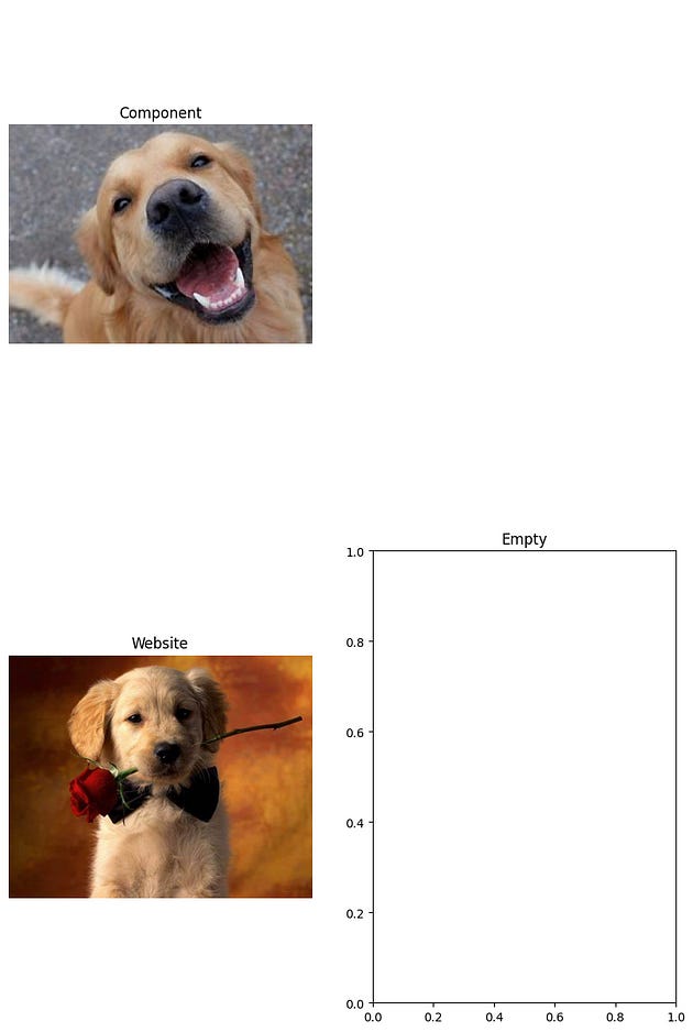

Steps 4- Image Transformations

Image transformations involve modifying images to enhance their features or make them more suitable for analysis. Common transformations include resizing, rotating, cropping, and more.

Common image transformation techniques include:

Color Spaces and Conversions
Turn our image object into a NumPy array
Rescale the images
Normalizing pixel values
Converting to grayscale
Histogram and Histogram equalization.
Data augmentation
Noise Reduction
Cropping Images
Morphological Transformations
Contour Detection and Analysis
Image Thresholding

1- Color Spaces and Conversions

It is used to change the mode of an image. The mode of an image defines the type and depth of a pixel in the image. Different modes support different types of images, and converting between them can be useful for various image processing tasks.

from PIL import Image

# Open an image file
image = Image.open('/content/gdrive/MyDrive/Datasets (1)/Image Preprocessing/dog.jfif')

plt.imshow(image)

# Convert to binary_scale
binary_image = image.convert('1')

plt.imshow(binary_image)

# Convert to grayscale
gray_image = image.convert('L')

plt.imshow(gray_image, cmap="gray")

print(np.array(binary_image))
print(np.array(gray_image))

# Convert to palette image
palette_image = image.convert('P')

plt.imshow(palette_image)

# Convert to RGBA
rgba_image = image.convert('RGBA')

plt.imshow(rgba_image)

# Convert to CMYK
cmyk_image = image.convert('CMYK')

plt.imshow(cmyk_image)

# Convert the image to grayscale
gray_img = cv2.cvtColor(img, cv2.COLOR_BGR2GRAY)

# Convert the image to HSV
hsv_img = cv2.cvtColor(img, cv2.COLOR_BGR2LAB)
luv_img = cv2.cvtColor(img, cv2.COLOR_BGR2LUV)

# Display the original, grayscale, and HSV images
plt.figure(figsize=(15, 15))
plt.subplot(2, 2, 1)
plt.imshow(cv2.cvtColor(img, cv2.COLOR_BGR2RGB))
plt.title('Original Image')
plt.axis('off')

plt.subplot(2, 2, 2)
plt.imshow(gray_img, cmap='gray')
plt.title('Grayscale Image')
plt.axis('off')

plt.subplot(2, 2, 3)
plt.imshow(hsv_img)
plt.title('HSV Image')
plt.axis('off')

plt.subplot(2, 2, 4)
plt.imshow(luv_img)
plt.title("LUV Image")
plt.axis("off")
plt.show()

2- Turn our image object into a NumPy array

# Turn our image object into a NumPy array
img_arr = np.array(img)

print("PIL Image:")
print("Type:", type(img))
print("Shape/Size:", img.size)
print()
print("After converting PIL image to Numpy Array:")
print("Type:", type(img_arr))
print("Shape/Size:", img_arr.shape)

PIL Image:
Type: <class 'PIL.JpegImagePlugin.JpegImageFile'>
Shape/Size: (640, 452)

After converting PIL image to Numpy Array:
Type: <class 'numpy.ndarray'>
Shape/Size: (452, 640, 3)

plt.figure(figsize=(12, 12))

plt.subplot(1, 4, 1)
plt.imshow(img_arr)

plt.subplot(1, 4, 2)
plt.imshow(img_arr[:,:,0], cmap='Reds')

plt.subplot(1, 4, 3)
plt.imshow(img_arr[:,:,1], cmap='Greens')

plt.subplot(1, 4, 4)
plt.imshow(img_arr[:,:,2], cmap='Blues')

3- Rescale the images

Resizing images changes their dimensions (height and width) to a standard size, which is crucial for ensuring uniform input sizes for machine learning models.s

This step is important because most neural networks require fixed input dimensions.

The images displayed above show us that the dataset has images with various scales. So, as a first preprocessing step, we will make sure that all images have the same height and width. When choosing an appropriate size we should keep in mind that bigger images correspond to higher computational requirements (both memory and operation wise).

As a first step we should figure out the dimensions of our images.

all_sizes = [io.imread(img).shape for img in all_images]

heights = [img_shape[0] for img_shape in all_sizes]
widths = [img_shape[1] for img_shape in all_sizes]

print(f"Minimum image height: {min(heights)}")
print(f"Maximum image height: {max(heights)}")
print()
print(f"Minimum image width: {min(widths)}")
print(f"Maximum image width: {max(widths)}")

We will resize the images to pixels using scikit-image (other shapes would be fine, too). The images won’t be cropped but up-sized or down-sized using interpolation.

Further, for simplicity, we will skip images that have less or more than 3 color channels (i.e. images whose mode is not RGB). As a quick reminder:

RGB is a 3-channel format corresponding to the channels red, green and blue. RGBA is a 4-channel format corresponding to red, green, blue and alpha. The alpha channel makes the color of the image transparant or translucent.

Note: make sure to create a folder named “resized_images”, otherwise the code below will raise an error!

resized_path = os.path.join(root_path, '/content/gdrive/MyDrive/Datasets (1)/Image Preprocessing/resized_images')

for img_path in all_images:
    # Create a new image name to save the resized image
    img_name = img_path.split('/')[-1]
    img_name = os.path.splitext(img_name)
    resized_name = img_name[0] + '_resized' + img_name[1]
    save_path = os.path.join(resized_path, resized_name)

    img = io.imread(img_path)

    if img.ndim != 3 or img.shape[2] != 3:
        continue

    resized_img = resize(img, output_shape=(256, 256))

    # Convert the resized image to uint8 before saving
    resized_img = (resized_img * 255).astype('uint8')  # Scale and convert to uint8

    io.imsave(save_path, resized_img)

all_images = glob.glob(resized_path + '/*')

# Plot a few images
fig = plt.figure(figsize=(10, 10))

i = 0
for img_path in all_images[:4]:
    img_arr = io.imread(img_path)
    i += 1
    ax = fig.add_subplot(2, 2, i)
    ax.imshow(img_arr)
    ax.set_title(f"Resized image example {i}")

Using OpenCV

# Resize the image to 224x224 pixels
resized_image = cv2.resize(image, (224, 224))

import cv2
import matplotlib.pyplot as plt

img = cv2.imread('images/nascom2.jpeg')
resized_img = cv2.resize(img, (200, 200))


plt.imshow(cv2.cvtColor(img, cv2.COLOR_BGR2RGB))
plt.title('Resized Image')
plt.axis("off")
plt.show()

Using PIL

# Resize the image to 224x224 pixels
resized_image = image.resize((224, 224))

4- Normalizing pixel values

Basically, normalizing pixel values means adjusting the intensity of pixels in an image to a set range like [0, 1] or [-1, 1]. This is done by dividing the pixel values by the maximum possible value (e.g., 255 for an 8-bit image). Normalization is important for making machine learning models train faster and more effectively by keeping input features on a consistent scale. This helps with stability and overall performance.

Normalizing pixel values has two steps:

Mean subtraction: in the case of images this often refers to subtracting the mean computed over all images from each pixel. The mean value can be computed over all three channels or for each channel individually. As described in the given link this has the “geometric interpretation of centering the cloud of data around the origin along every dimension”.

Divide by standard deviation: This step is not strictly necessary for images because the relative pixel scales are already approximately equal. Nevertheless, we will include this step for completeness.

# To compute the mean and standard deviation over all images
# we need to combine them in one big array
big_list = []

for img_path in all_images:
    big_list.append(io.imread(img_path))

all_imgs = np.array(big_list)

# The image pixels are uint8. To compute a mean we
# convert the pixel values to floats
all_imgs_float = img_as_float(all_imgs)

# Mean subtraction
mean = np.mean(all_imgs_float, axis=0)
all_imgs_float -= mean

# Dividing by standard deviation
std = np.std(all_imgs_float, axis=0)
all_imgs_float /= std
fig = plt.figure(figsize=(12, 12))

for i in range(9):
    ax = fig.add_subplot(3, 3, i+1)
    ax.imshow(all_imgs_float[i])
    ax.set_title(f"Normalized image example {i+1}")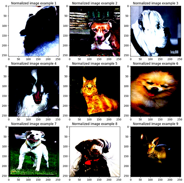

Using OpenCV

# Normalize pixel values to [0, 1]
normalized_image = image / 255.0

5- Converting to grayscale

Converting color images to grayscale can simplify your image data and reduce computational needs for some algorithms.

Converting between color spaces: You may need to convert images between color spaces like RGB, BGR, HSV, and Grayscale. This can be done with OpenCV or Pillow. For example, to convert BGR to Grayscale in OpenCV, use:

Converting the images to grayscale is very easy with scikit-image.

gray_images = rgb2gray(all_imgs)

fig = plt.figure(figsize=(10, 10))
for i in range(4):
    ax = fig.add_subplot(2, 2, i+1)
    ax.imshow(gray_images[i], cmap='gray')
    ax.set_title(f"Grayscale image example {i+1}")

gray = cv2.cvtColor (image, cv2.COLOR_BGR2GRAY)

Or to convert RGB to HSV in Pillow:

image = image.convert('HSV')

6-Histogram and Histogram equalization.

Histogram

Image preprocessing is an important step in many computer vision tasks, and one of the common techniques used is histogram equalization.

Def: In image processing, a histogram is a graphical representation that depicts the distribution of pixel intensities in an image.

It’s essentially a bar graph where:

• The x-axis represents the intensity values (usually ranging from 0 to 255 for grayscale images).

• The y-axis represents the number of pixels with a particular intensity value.

By analyzing the histogram, you can gain valuable insights about the image’s:

• Contrast: A flat histogram indicates low contrast, while peaks and valleys suggest higher contrast.

• Brightness: A histogram skewed towards the left indicates a dark image, while a skew towards the right indicates a brighter image.

Calculating Histograms with OpenCV

OpenCV provides the cv2.calcHist function to compute histograms:

Step-by-Step Explanation

1. Load the Image: First, load the image you want to preprocess.

2. Convert to Grayscale (Optional): Histogram equalization is usually applied to grayscale images. If your image is in color, you may want to convert it to grayscale.

3. Apply Histogram Equalization: Use a function like cv2.equalizeHist() from the OpenCV library to apply histogram equalization.

4. Display or Save the Processed Image: Finally, display the equalized image or save it for later use.

from google.colab import drive
drive.mount('/content/gdrive')

# Calculate the histogram of the grayscale image

import cv2
import matplotlib.pyplot as plt

# Load an image from file (ensure the path is correct for your system)
image_path = '/content/gdrive/MyDrive/Datasets (1)/Image Preprocessing/dog.jfif'
img = cv2.imread(image_path)

# Convert the image to grayscale
gray_img = cv2.cvtColor(img, cv2.COLOR_BGR2GRAY)

# Calculate the histogram of the grayscale image
hist = cv2.calcHist([gray_img], [0], None, [256], [0, 256])

# Display the original grayscale image and its histogram
plt.figure(figsize=(15, 5))

# Display the grayscale image
plt.subplot(1, 2, 1)
plt.imshow(gray_img, cmap='gray')
plt.title('Original Grayscale Image')
plt.axis('off')

# Display the histogram
plt.subplot(1, 2, 2)
plt.plot(hist, color='black')
plt.title('Histogram of Original Image')
plt.xlabel('Pixel Intensity')
plt.ylabel('Frequency')
plt.grid(True)

# Show the plots
plt.tight_layout()
plt.show()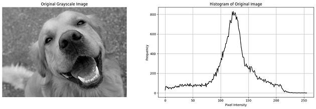

Histogram Equalization

Histogram equalization is a method that improves the contrast of an image by adjusting the intensity distribution.

• Histogram equalization is an image processing technique that enhances the contrast of an image by redistributing the pixel intensities.

• It aims to create a more uniform distribution of intensity values in the image’s histogram.

• This process often improves the visibility of details in low-contrast images.

How Histogram Equalization Works (Self Learning)

1. Calculate Histogram: First, the histogram of the image is computed, as explained earlier.

2. Cumulative Distribution Function (CDF): The CDF is calculated from the histogram. The CDF represents the probability of a pixel having an intensity value less than or equal to a specific value.

3. Intensity Remapping: Each pixel’s intensity is then remapped based on the CDF. This essentially stretches out the distribution of intensity values, making areas with low contrast more distinct.

import cv2
import matplotlib.pyplot as plt

# Step 1: Load the image (Make sure to provide the correct path)
img = cv2.imread('/content/gdrive/MyDrive/Datasets (1)/Image Preprocessing/dog.jfif')

# Step 2: Convert to Grayscale (if the image is not already in grayscale)
gray_image = cv2.cvtColor(img, cv2.COLOR_BGR2GRAY)

# Step 3: Apply Histogram Equalization
equalized_image = cv2.equalizeHist(gray_image)

# Step 4: Display the Original and Equalized Images
plt.figure(figsize=(10, 5))

# Original Image
plt.subplot(1, 2, 1)
plt.title('Original Image')
plt.imshow(gray_image, cmap='gray')
plt.axis('off')

# Equalized Image
plt.subplot(1, 2, 2)
plt.title('Equalized Image')
plt.imshow(equalized_image, cmap='gray')
plt.axis('off')

plt.show()

import cv2
import matplotlib.pyplot as plt

# Load an image from file (ensure the path is correct for your system)
image_path = '/content/gdrive/MyDrive/Datasets (1)/Image Preprocessing/dog.jfif'
img = cv2.imread(image_path)

# Convert the image to grayscale
gray_img = cv2.cvtColor(img, cv2.COLOR_BGR2GRAY)

# Calculate the histogram of the grayscale image
hist = cv2.calcHist([gray_img], [0], None, [256], [0, 256])

# Equalize the histogram
equalized_img = cv2.equalizeHist(gray_img)

# Display the original and equalized images and their histograms
plt.figure(figsize=(15, 10))

# Display the original grayscale image
plt.subplot(2, 2, 1)
plt.imshow(gray_img, cmap='gray')
plt.title('Original Grayscale Image')
plt.axis('off')

# Display the histogram of the original image
plt.subplot(2, 2, 2)
plt.plot(hist, color='black')
plt.title('Histogram of Original Image')
plt.xlabel('Pixel Intensity')
plt.ylabel('Frequency')
plt.grid(True)

# Display the equalized grayscale image
plt.subplot(2, 2, 3)
plt.imshow(equalized_img, cmap='gray')
plt.title('Equalized Image')
plt.axis('off')

# Display the histogram of the equalized image
plt.subplot(2, 2, 4)
plt.plot(cv2.calcHist([equalized_img], [0], None, [256], [0, 256]), color='black')
plt.title('Histogram of Equalized Image')
plt.xlabel('Pixel Intensity')
plt.ylabel('Frequency')
plt.grid(True)

# Show the plots
plt.tight_layout()
plt.show()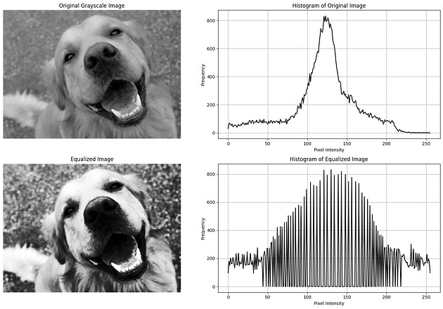

Important Considerations

• Histogram equalization can sometimes introduce noise or artifacts into the image, especially with images that have low inherent contrast.

• It’s a global contrast enhancement technique, meaning it applies the same transformation to the entire image

7- Data augmentation

Image augmentation is a technique to artificially increase the size of a dataset by creating modified versions of images. Common augmentations include rotation, flipping, and zooming.

First of all: why do we need data augmentation?

The performance of a machine learning algorithm depends heavily on the amount and quality of the data it is trained with. In most cases, the more data a machine learning algorithm has access to, the more effective it can be. However, most of the time, we only have access to a small amount of data with sufficient quality. So, if we augment our dataset in a useful way we can improve the performance of our model without having to gather a larger dataset.

Furthermore, augmenting the dataset can make our model more robust. For example, consider the task of image classification. Let’s say we want to classify the breed of dog/cat shown in each image of our dataset. Our training set will contain only a limited amount of images each breed, and each breed will be displayed in a limited set of conditions. However, our test set (or real world application) may contain images of dogs and cats in a large variety of conditions. The images could be taken from various angles, locations, lighting conditions, etc. By augmenting our training set with small variations of the original images, we can allow our model to account for such variations.

Images can be augmented in various ways, for example using:

1- rotation

2- translation

3- rescaling

4- lipping

5- stretching etc.

scikit-image

Most of these tasks can be performed easily with scikit-image or one of the other image processing libraries. Let’s look at rotation as an example.

fig = plt.figure(figsize=(10, 10))

for i in range(4):
    random_angle = np.random.randint(low=0, high=360)
    rotated_image = rotate(all_imgs[i], angle=random_angle)
    ax = fig.add_subplot(2, 2, i+1)
    ax.imshow(rotated_image)
    ax.set_title(f"Randomly rotated image example {i+1}")

Using TensorFlow

TensorFlow provides a high-level API for image augmentation.

from tensorflow.keras.preprocessing.image import ImageDataGenerator

# Create an image data generator with augmentation
datagen = ImageDataGenerator(
    rotation_range=40,
    width_shift_range=0.2,
    height_shift_range=0.2,
    shear_range=0.2,
    zoom_range=0.2,
    horizontal_flip=True,
    fill_mode='nearest'
)

# Assuming 'image' is a numpy array of shape (height, width, channels)
image = image.reshape((1, ) + image.shape)  # Reshape image for the generator

# Generate batches of augmented images
for batch in datagen.flow(image, batch_size=1):
    augmented_image = batch[0]
    break  # To generate one augmented image

Open CV

 Define the rotation matrix

center = (img.shape[1] // 2, img.shape[0] // 2)
rotation_matrix = cv2.getRotationMatrix2D(center, -30, .80)

# Convert the image from BGR to RGB# Rotate the image
rotated_img = cv2.warpAffine(img, rotation_matrix, (img.shape[1], img.shape[0]))

# Convert the image from BGR to RGB
rotated_img_rgb = cv2.cvtColor(rotated_img, cv2.COLOR_BGR2RGB)

# Display the original and rotated images
plt.figure(figsize=(10, 5))
plt.subplot(1, 2, 1)
plt.imshow(cv2.cvtColor(img, cv2.COLOR_BGR2RGB))
plt.title('Original Image')
plt.axis('off')

plt.subplot(1, 2, 2)
plt.imshow(rotated_img_rgb)
plt.title('Rotated Image')
plt.axis('off')

plt.show()

8- Noise Reduction

Reducing noise can help improve the clarity of the image and the performance of the model.

a kernel (also known as a filter or mask) is a small matrix used to perform operations on an image. The kernel is a fundamental concept that enables a wide range of image manipulations, from Filtering (i.e. blurring and sharpening to edge detection.)

What is a Kernel?

1. Definition:

• A kernel is a grid of numbers, usually a small square matrix (e.g., 3x3, 5x5), that slides over an image to apply a specific effect or extract features.

1. Function:

• Convolution: The process of applying a kernel to an image is called convolution. This involves placing the kernel on a part of the image, performing element-wise multiplication between the kernel values and the corresponding image pixel values, and summing the results to produce a new pixel value in the output image.

Smoothing, blurring, and filtering techniques can be applied to remove unwanted noise from images. The GaussianBlur () and medianBlur () methods are commonly used for this.

Filtering Techniques

Filtering techniques involve modifying images to enhance or detect specific features. Common filters include blurring, sharpening, and edge detection.

1. Blurring Filters

Blurring filters are used to reduce noise and unwanted details in an image, creating a smoother appearance. Here are some common types of blurring:

• Averaging Blur: This is a simple and fast blurring technique that replaces each pixel with the average intensity of its neighbors within a specified kernel (usually a square). It’s implemented using the cv2.blur function:

from google.colab import drive
drive.mount('/content/gdrive')

import cv2
import matplotlib.pyplot as plt

img = cv2.imread('/content/gdrive/MyDrive/Datasets (1)/Image Preprocessing/dog.jfif')

kernel_size = 15
# Performed Averaging bluy
blurred_avg = cv2.blur(img, (kernel_size, kernel_size))

blurred_avg = cv2.cvtColor(blurred_avg, cv2.COLOR_BGR2RGB)
plt.imshow(blurred_avg)
plt.title('Averaging Blur Image')
plt.axis('off')
plt.show()

import cv2

# Assuming 'all_imgs' is a list of images, iterate over each image:
denoised_images = []
for img in all_imgs:
    denoised_image = cv2.GaussianBlur(img, (5, 5), 0)
    denoised_images.append(denoised_image)

fig = plt.figure(figsize=(10, 10))

for i in range(4):
    random_angle = np.random.randint(low=0, high=360)
    rotated_image = rotate(denoised_images[i], angle=random_angle)
    ax = fig.add_subplot(2, 2, i+1)
    ax.imshow(rotated_image)
    ax.set_title(f"Randomly rotated image example {i+1}")

• Gaussian Blur: Similar to averaging, but uses a Gaussian kernel that assigns higher weights closer to the center, resulting in a smoother blur with less pronounced edges. Use cv2.GaussianBlur:

blurred_gauss = cv2.GaussianBlur(img, (kernel_size, kernel_size), 0)


blurred_gauss = cv2.cvtColor(blurred_gauss, cv2.COLOR_BGR2RGB)
plt.imshow(blurred_gauss)
plt.title('Gaussian  Blur')
plt.axis('off')
plt.show()

• Median Blur: This technique is effective for removing salt-and-pepper noise (randomly distributed black and white pixels) by replacing each pixel with the median intensity value in its neighborhood. Use cv2.medianBlur:

blurred_median = cv2.medianBlur(img, kernel_size)

blurred_median = cv2.cvtColor(blurred_median, cv2.COLOR_BGR2RGB)

plt.imshow(blurred_median)
plt.title('Median  Blur')
plt.axis('off')
plt.show()

2. Sharpening Filters

Sharpening filters enhance edges and high-frequency details in an image, making them appear more crisp and defined. Here’s a common approach:

• Laplacian Filter: This filter highlights edges by emphasizing intensity differences between neighboring pixels. Use cv2.Laplacian:

import numpy as np

sharpened = cv2.Laplacian(img, cv2.CV_8U)  # Convert to 8-bit unsigned

plt.imshow(sharpened)
plt.title('Sharpening')
plt.axis('off')
plt.show()

3. Edge Detection Filters

Edge detection filters identify and localize boundaries between objects in an image. Here are two popular methods:

• Sobel Operator: The Sobel filter calculates the gradient of the image intensity at each pixel, which indicates how abrupt the change is at that point. It uses two 3x3 convolution kernels, one for detecting changes in the horizontal direction Gx and one for detecting changes in the vertical direction

sobelx = cv2.Sobel(img, cv2.CV_8U, 1, 0, ksize=3)  # Horizontal edges
sobely = cv2.Sobel(img, cv2.CV_8U, 0, 1, ksize=3)  # Vertical edges

plt.imshow(sobelx)
plt.title('Median  Blur')
plt.axis('off')
plt.show()

Canny Edge Detection Algorithm(self reading)

# Set the thresholds for the Canny edge detector

# Threshold values btw 0, 255
threshold1 = 200  # Lower threshold
threshold2 = 250  # Upper threshold


edges = cv2.Canny(img, threshold1, threshold2)  # Set appropriate thresholds
edges_rgb = cv2.cvtColor(edges, cv2.COLOR_GRAY2RGB)

plt.imshow(edges_rgb)
plt.title('Median  Blur')
plt.axis('off')
plt.show()

# Apply a Gaussian blur
blurred_img = cv2.GaussianBlur(img, (15, 15), 0)

# Apply a sharpening filter
kernel = np.array([[0, -1, 0], [-1, 5, -1], [0, -1, 0]])
sharpened_img = cv2.filter2D(img, -1, kernel)

# Apply the Canny edge detector
edges = cv2.Canny(img, 100, 200)

# Convert the images from BGR to RGB
blurred_img_rgb = cv2.cvtColor(blurred_img, cv2.COLOR_BGR2RGB)
sharpened_img_rgb = cv2.cvtColor(sharpened_img, cv2.COLOR_BGR2RGB)
edges_rgb = cv2.cvtColor(edges, cv2.COLOR_GRAY2RGB)

# Display the original, blurred, sharpened, and edge-detected images
plt.figure(figsize=(20, 5))
plt.subplot(1, 4, 1)
plt.imshow(cv2.cvtColor(img, cv2.COLOR_BGR2RGB))
plt.title('Original Image')
plt.axis('off')

plt.subplot(1, 4, 2)
plt.imshow(blurred_img_rgb)
plt.title('Blurred Image')
plt.axis('off')

plt.subplot(1, 4, 3)
plt.imshow(sharpened_img_rgb)
plt.title('Sharpened Image')
plt.axis('off')

plt.subplot(1, 4, 4)
plt.imshow(edges_rgb)
plt.title('Edges Detected')
plt.axis('off')

plt.show()

9. Cropping Images

Cropping involves extracting a specific rectangular region from an image. This can be useful for focusing on regions of interest.

# Define the cropping coordinates (start_row, start_col, end_row, end_col)
start_row, start_col = 80, 140
end_row, end_col = 350, 1410

# Crop the image
cropped_img = img[start_row:end_row, start_col:end_col]

# Convert the image from BGR to RGB
cropped_img_rgb = cv2.cvtColor(cropped_img, cv2.COLOR_BGR2RGB)

# Display the original and cropped images
plt.figure(figsize=(10, 5))
plt.subplot(1, 2, 1)
plt.imshow(cv2.cvtColor(img, cv2.COLOR_BGR2RGB))
plt.title('Original Image')
plt.axis('off')

plt.subplot(1, 2, 2)
plt.imshow(cropped_img_rgb)
plt.title('Cropped Image')
plt.axis('off')

plt.show()

10- Morphological Transformations

Morphological transformations are a set of operations that process images based on shapes. These operations apply a structuring element to an input image and generate an output image.

Erosion
Dilation
Opening
Closing

Erosion

Erosion reduces the boundaries of the foreground object. It is useful for removing small white noises and isolating individual elements. you can apply erosion using the cv2.erode() function.

from google.colab import drive
drive.mount('/content/gdrive')

import cv2
import numpy as np
import matplotlib.pyplot as plt

# Load the image
image = cv2.imread('/content/gdrive/MyDrive/Datasets (1)/Image Preprocessing/dog.jfif')
# Create a structuring element
kernel = np.ones((6,6), np.uint8)

# Apply erosion
erosion = cv2.erode(image, kernel, iterations = 1)

# Display the result
plt.figure(figsize=(15, 10))
plt.subplot(121), plt.imshow(image, cmap='gray'), plt.title('Original Image')
plt.axis('off')
plt.subplot(122), plt.imshow(erosion, cmap='gray'), plt.title('Eroded Image')
plt.axis('off')
plt.show()

Dilation

Dilation increases the object area and is useful for connecting broken parts of an object. the cv2.dilate() function is used to apply dilation.

# Apply dilation
dilation = cv2.dilate(image, kernel, iterations = 1)

# Display the result
plt.figure(figsize=(15, 10))
plt.subplot(121), plt.imshow(image, cmap='gray'), plt.title('Original Image'), plt.axis('off')
plt.subplot(122), plt.imshow(dilation, cmap='gray'), plt.title('Dilated Image'), plt.axis('off')
plt.show()

Opening

Opening is a combination of erosion followed by dilation. It is useful for removing noise. The cv2.morphologyEx() function is used to apply opening. and the cv2.MORPH_OPEN flag is used to specify opening.

# Apply opening
opening = cv2.morphologyEx(image, cv2.MORPH_OPEN, kernel)

# Display the result
plt.figure(figsize=(15, 10))
plt.subplot(121), plt.imshow(image, cmap='gray'), plt.title('Original Image'), plt.axis('off')
plt.subplot(122), plt.imshow(opening, cmap='gray'), plt.title('Opened Image'), plt.axis('off')
plt.show()

Closing

Closing is a combination of dilation followed by erosion. It is useful for closing small holes inside the foreground objects. The cv2.morphologyEx() function is used to apply closing. and the cv2.MORPH_CLOSE flag is used to specify closing.

# Apply closing
closing = cv2.morphologyEx(image, cv2.MORPH_CLOSE, kernel)

# Display the result
plt.figure(figsize=(15, 10))
plt.subplot(121), plt.imshow(image, cmap='gray'), plt.title('Original Image'), plt.axis('off')
plt.subplot(122), plt.imshow(closing, cmap='gray'), plt.title('Closed Image'), plt.axis('off')
plt.show()

10- Contour Detection and Analysis

Contours can be explained simply as a curve joining all the continuous points (along the boundary), having the same color or intensity. The contours are a useful tool for shape analysis and object detection and recognition.

to find contours in an image, you can use the cv2.findContours() function. This function returns a list of contours and a hierarchy. The contours are a Python list of all the contours in the image. Each individual contour is a Numpy array of (x, y) coordinates of boundary points of the object.

# open the image
image = cv2.imread('/content/gdrive/MyDrive/Datasets (1)/Image Preprocessing/dog.jfif')

# Convert the image to grayscale
gray = cv2.cvtColor(image, cv2.COLOR_BGR2GRAY)

# Apply thresholding
ret, thresh = cv2.threshold(gray, 90, 255, 0)

# Find contours
contours, hierarchy = cv2.findContours(thresh, cv2.RETR_TREE, cv2.CHAIN_APPROX_SIMPLE)

image = cv2.cvtColor(image, cv2.COLOR_BGR2RGB) # Convert the image to RGB space

print(len(contours))
# Draw contours with different colors based on hierarchy
contour_image = image.copy()
for i in range(len(contours)):
    if hierarchy[0][i][3] == -1:
        color = (5, 0, 250)  # Blue color for contours with no parent
    else:
        color = (0, 255, 0)  # Green color for contours with parent
    contour_image = cv2.drawContours(contour_image, contours, i, color, 1)

# Display the result
plt.figure(figsize=(15, 10))
plt.imshow(contour_image)
plt.title('Contours')
plt.axis('off')
plt.show()

11. Image Thresholding

Image thresholding is a simple yet effective technique for segmenting images. It is used to create binary images from grayscale images. The thresholding operation compares each pixel of an image with a predefined threshold value. If the pixel value is greater than the threshold, it is assigned one value (usually white), and if it is less than the threshold, it is assigned another value (usually black).

1- Simple Thresholding

Simple thresholding is the most basic form of thresholding. It is used to create a binary image from a grayscale image. The cv2.threshold() function is used to apply simple thresholding.

# Apply simple thresholding
ret, thresh = cv2.threshold(gray, 147, 255, cv2.THRESH_BINARY)

# Display the result
plt.figure(figsize=(15, 10))
plt.subplot(121), plt.imshow(gray, cmap='gray'), plt.title('Original Image'), plt.axis('off')
plt.subplot(122), plt.imshow(thresh, cmap='gray'), plt.title('Thresholded Image'), plt.axis('off')
plt.show()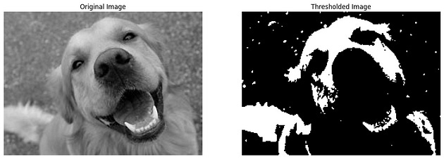

Adaptive Thresholding

Adaptive thresholding is used when the image has different lighting conditions in different areas. It calculates the threshold for a small region of the image. The cv2.adaptiveThreshold() function is used to apply adaptive thresholding.

The parameters for cv2.adaptiveThreshold are:

• gray : The input image

• maxValue : The maximum intensity value that can be assigned to a pixel (usually 255)

• adaptiveMethod : The method used to calculate the threshold value (Chooses between cv2.ADAPTIVE_THRESH_MEAN_C or cv2.ADAPTIVE_THRESH_GAUSSIAN_C.)

• thresholdType : The type of thresholding operation

• blockSize : The size of the neighborhood area used to calculate the threshold value

• C : A constant value subtracted from the calculated threshold value

# Apply adaptive thresholding
thresh2 = cv2.adaptiveThreshold(gray, 255, cv2.ADAPTIVE_THRESH_MEAN_C, cv2.THRESH_BINARY, 5, 2)

# Display the result
plt.figure(figsize=(15, 10))
plt.imshow(thresh2, cmap='gray')
plt.title('Adaptive Thresholding')
plt.axis('off')
plt.show()

Otsu’s Binarization

# Apply Otsu's binarization
ret2, thresh3 = cv2.threshold(gray, 0, 255, cv2.THRESH_BINARY + cv2.THRESH_OTSU)

# Display the result
plt.figure(figsize=(15,10))
plt.imshow(thresh3, cmap='gray')
plt.title('Otsu\'s Binarization')
plt.axis('off')
plt.show()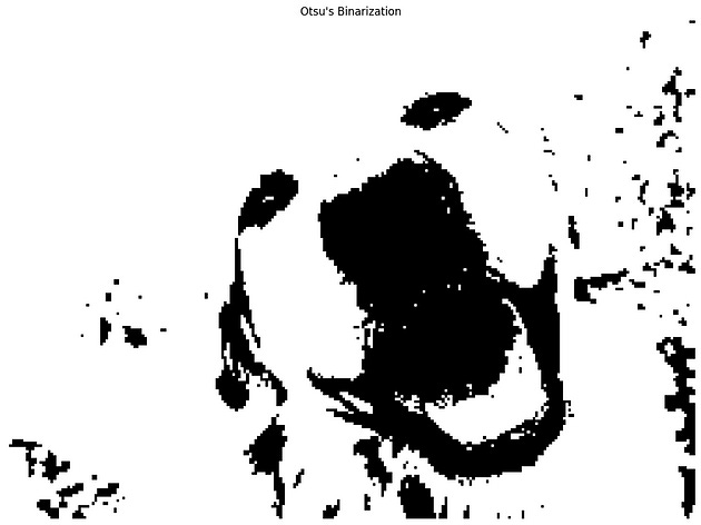

Steps 5- Feature Detection and Description

Understanding Features

Features in computer vision refer to the distinct, easily identifiable structures within an image, such as corners, edges, and blobs. These features are used for tasks such as object recognition, image stitching, and motion tracking.

Edge Detection Techniques
Keypoint Detection and Description

Edge Detection Techniques

Edge detection is a technique used to identify the boundaries within an image, which helps to highlight the significant features.

Sobel Edge Detection
Canny Edge Detection

1. Sobel Edge Detection: The Sobel operator is used to detect edges in an image by calculating the gradient magnitude at each pixel.

from google.colab import drive
drive.mount('/content/gdrive')

import cv2
import numpy as np
import matplotlib.pyplot as plt

# Load the image
image = cv2.imread('/content/gdrive/MyDrive/Datasets (1)/Image Preprocessing/dog.jfif', cv2.IMREAD_GRAYSCALE)

# Apply Sobel operator
sobel_x = cv2.Sobel(image, cv2.CV_64F, 1, 0, ksize=5)
sobel_y = cv2.Sobel(image, cv2.CV_64F, 0, 1, ksize=5)

# Calculate the gradient magnitude
sobel_combined = cv2.magnitude(sobel_x, sobel_y)

# Display the results using matplotlib
plt.figure(figsize=(12, 12))
plt.subplot(2, 2, 1)
plt.imshow(sobel_x, cmap='gray')
plt.title('Sobel X')
plt.axis("off")
plt.subplot(2, 2, 2)
plt.imshow(sobel_y, cmap='gray')
plt.axis("off")
plt.title('Sobel Y')
plt.subplot(2, 2, 3)
plt.imshow(sobel_combined, cmap='gray_r')
plt.title('Sobel Combined')
plt.axis("off")
plt.subplot(2,2,4)
plt.imshow(image, cmap="gray")
plt.axis("off")
plt.title("Original")
plt.show()

Canny Edge Detection: The Canny edge detection algorithm is a multi-stage process that includes noise reduction, gradient calculation, non-maximum suppression, and edge tracking by hysteresis.

# Apply Canny edge detection
canny_edges = cv2.Canny(image, 90, 200)

# Display the result using matplotlib
plt.figure(figsize=(6, 4))
plt.imshow(canny_edges, cmap='gray_r')
plt.title('Canny Edges')
plt.show()

Keypoint Detection and Description

Keypoints are the specific points in an image that are used to define its significant features. Descriptors are the vectors that describe the local region around each keypoint.

SIFT
SURF
ORB

1. SIFT (Scale-Invariant Feature Transform): SIFT is a powerful algorithm that detects and describes local features in images.

from google.colab import drive
drive.mount('/content/gdrive')

import cv2
import matplotlib.pyplot as plt

# Load the image
image = cv2.imread('/content/gdrive/MyDrive/Datasets (1)/Image Preprocessing/dog.jfif')
gray_image = cv2.cvtColor(image, cv2.COLOR_BGR2GRAY)

# Create SIFT detector object
sift = cv2.SIFT_create()

# Detect keypoints and descriptors
keypoints, descriptors = sift.detectAndCompute(gray_image, None)

# Draw keypoints on the image
sift_image = cv2.drawKeypoints(image, keypoints, None)

# Display the result using matplotlib
plt.figure(figsize=(10, 10))
plt.imshow(cv2.cvtColor(sift_image, cv2.COLOR_BGR2RGB))
plt.title('SIFT Keypoints')
plt.axis("off")
plt.show()

1. SURF (Speeded-Up Robust Features): SURF is a fast approximation of SIFT, useful for real-time applications.

# Create SURF detector object
sift = cv2.SIFT_create()

# Detect keypoints and descriptors
kp = sift.detect(gray_image,None)

# Draw keypoints on the image
surf_image = cv2.drawKeypoints(gray_image,kp,image)

# Display the result using matplotlib
plt.figure(figsize=(10, 10))
plt.imshow(cv2.cvtColor(surf_image, cv2.COLOR_BGR2RGB))
plt.title('SURF Keypoints')
plt.axis("off")
plt.show()

1. ORB (Oriented FAST and Rotated BRIEF): ORB is an efficient alternative to SIFT and SURF, providing fast and accurate keypoint detection and description.

# Create ORB detector object
orb = cv2.ORB_create()

# Detect keypoints and descriptors
keypoints, descriptors = orb.detectAndCompute(gray_image, None)

# Draw keypoints on the image
orb_image = cv2.drawKeypoints(image, keypoints, None)

# Display the result using matplotlib
plt.figure(figsize=(10, 10))
plt.imshow(cv2.cvtColor(orb_image, cv2.COLOR_BGR2RGB))
plt.title('ORB Keypoints')
plt.axis('off')
plt.show()

Steps 6- Hough Transform for Shape Detection

The Hough Transform is a powerful technique used in image processing and computer vision for detecting shapes, such as lines and circles, within an image. The method works by transforming points in an image space to a parameter space where shapes can be detected as peaks. Below are explanations of how the Hough Line Transform and the Hough Circle Transform work.

Hough Line Transform

Concept:

The Hough Line Transform is used to detect straight lines in an image. The basic idea is to transform the points in the image space (x, y) into a parameter space defined by the line parameters. In the case of a line, these parameters are typically the distance from the origin (rho) and the angle from the x-axis (theta).

Mathematical Representation:

A line in Cartesian coordinates can be represented as: y=mx+b where m is the slope and b is the y-intercept.

Alternatively, in the Hough Transform, a line can be represented in polar coordinates as: ρ=xcos⁡(θ)+ysin⁡(θ) where:

• ρ is the distance from the origin to the closest point on the line.

• θ is the angle between the x-axis and the line connecting the origin with this closest point.

Algorithm Steps:

1. Edge Detection: Apply an edge detector (e.g., Canny) to find the edges in the image.

2. Transform Points: For each edge point (x,y), compute the values of ρ for different values of θ.

3. Accumulator Space: Vote in an accumulator space (a 2D array) where each cell corresponds to a specific (ρ,θ) pair. The value in each cell represents the number of points that are consistent with that line.

4. Detect Peaks: Identify peaks in the accumulator space, which correspond to the most prominent lines in the image.

5. Draw Lines: Convert the (ρ,θ) values back to Cartesian coordinates and draw the lines on the image.

from google.colab import drive
drive.mount('/content/gdrive')

import cv2
import numpy as np
import matplotlib.pyplot as plt

# Draw the lines represented in the hough accumulator on the original image
def drawhoughLinesOnImage(image, houghLines):
    for line in houghLines:
        for rho,theta in line:
            a = np.cos(theta)
            b = np.sin(theta)
            x0 = a*rho
            y0 = b*rho
            x1 = int(x0 + 1000*(-b))
            y1 = int(y0 + 1000*(a))
            x2 = int(x0 - 1000*(-b))
            y2 = int(y0 - 1000*(a))
            
            cv2.line(image,(x1,y1),(x2,y2),(0,255,0), 2)   

# Different weights are added to the image to give a feeling of blending
def blend_images(image, final_image, alpha=0.7, beta=1., gamma=0.):
    return cv2.addWeighted(final_image, alpha, image, beta,gamma)

image = cv2.imread("/content/gdrive/MyDrive/Datasets (1)/Image Preprocessing/hug1.png") # load image in grayscale
gray_image = cv2.cvtColor(image, cv2.COLOR_RGB2GRAY)
blurredImage = cv2.GaussianBlur(gray_image, (5, 5), 0)
edgeImage = cv2.Canny(blurredImage, 50, 120)

# Detect points that form a line
dis_reso = 1 # Distance resolution in pixels of the Hough grid
theta = np.pi /180 # Angular resolution in radians of the Hough grid
threshold = 170# minimum no of votes

houghLines = cv2.HoughLines(edgeImage, dis_reso, theta, threshold)

houghLinesImage = np.zeros_like(image) # create and empty image

drawhoughLinesOnImage(houghLinesImage, houghLines) # draw the lines on the empty image
orginalImageWithHoughLines = blend_images(houghLinesImage,image) # add two images together, using image blending


plt.figure(figsize=(12, 12))
plt.subplot(2, 1, 1)
plt.imshow(image, cmap='gray')
plt.title('Original Image')
plt.axis("off")
plt.subplot(2, 1, 2)
plt.imshow(edgeImage, cmap='gray')
plt.axis("off")
plt.title('Hough Image')
plt.show()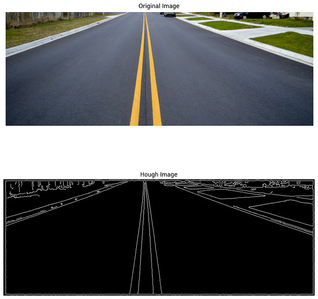

Steps 7- Template Matching

Template matching is a classical computer vision technique used to locate a specific pattern or object within an image. This technique involves sliding a template image over the target image to find the regions where the template matches the target best. It’s commonly used for object detection, image alignment, and image recognition tasks.

Key Concepts and Steps

1. Template Image:

• The template image is a smaller image or pattern that you want to find within a larger target image. This template can be a simple shape, character, or object.

1. Sliding Window:

• The template is moved (slid) across the target image, and at each position, a similarity measure is computed between the template and the region of the target image currently under the template.

1. Similarity Measures:

• Several methods can be used to calculate the similarity between the template and the target image region:

• Normalized Cross-Correlation (NCC): Measures how well the template matches the image region. High values indicate a good match.

• Sum of Squared Differences (SSD): Measures the sum of squared differences between the template and the image region.

• Sum of Absolute Differences (SAD): Measures the sum of absolute differences between the template and the image region.

• Correlation Coefficient: Measures the correlation between the template and the image region.

1. Finding the Best Match

• After computing similarity scores for all positions, the location with the highest (or lowest, depending on the method) similarity score is considered the best match

1. Draw Bounding Box:

• A bounding box can be drawn around the detected template location in the target image to visualize the match.

from google.colab import drive
drive.mount('/content/gdrive')

import cv2
import numpy as np
import matplotlib.pyplot as plt # Import the necessary library

import cv2
import numpy as np

# Load the target image and the template image
target_image = cv2.imread('/content/gdrive/MyDrive/Datasets (1)/Image Preprocessing/main.jpeg')
template_image = cv2.imread('/content/gdrive/MyDrive/Datasets (1)/Image Preprocessing/sub.jpeg')

# Convert images to grayscale
target_gray = cv2.cvtColor(target_image, cv2.COLOR_BGR2GRAY)
template_gray = cv2.cvtColor(template_image, cv2.COLOR_BGR2GRAY)

# Perform template matching
result = cv2.matchTemplate(target_gray, template_gray, cv2.TM_CCOEFF_NORMED)

# Find the location of the best match
min_val, max_val, min_loc, max_loc = cv2.minMaxLoc(result)

# Draw a rectangle around the detected template
template_height, template_width = template_gray.shape
top_left = max_loc
bottom_right = (top_left[0] + template_width, top_left[1] + template_height)
cv2.rectangle(target_image, top_left, bottom_right, (0, 255, 0), 2)

# Display output
plt.figure(figsize=(10, 10))
plt.imshow(cv2.cvtColor(target_image, cv2.COLOR_BGR2RGB))
plt.title('Templating')
plt.axis("off")
plt.show()

import cv2
import matplotlib.pyplot as plt
import numpy as np


# Load the target image and the template image
target_image = cv2.imread('/content/gdrive/MyDrive/Datasets (1)/Image Preprocessing/main.jpeg')
template_image = cv2.imread('/content/gdrive/MyDrive/Datasets (1)/Image Preprocessing/sub.jpeg')

# Convert images to grayscale
target_gray = cv2.cvtColor(target_image, cv2.COLOR_BGR2GRAY)
template_gray = cv2.cvtColor(template_image, cv2.COLOR_BGR2GRAY)
w, h = template_gray.shape[::-1]

# Perform template matching
result = cv2.matchTemplate(target_gray, template_gray, cv2.TM_CCOEFF_NORMED)

threshold = 0.9
loc = np.where( result >= threshold)

for pt in zip(*loc[::-1]):
    cv2.rectangle(target_image, pt, (pt[0] + w, pt[1] + h), (255,255,255), 1)
 
# Display output
plt.figure(figsize=(10, 10))
plt.imshow(cv2.cvtColor(target_image, cv2.COLOR_BGR2RGB))
plt.title('Templating')
plt.axis("off")
plt.show()

Key Points

1. Template Size:

• The size of the template image is crucial. A template that’s too small may not accurately capture the pattern, while a template that’s too large might not fit the target image properly.

1. Template Matching Methods:

• OpenCV provides several methods for template matching (cv2.matchTemplate), each suited to different types of images and templates. Choose the method that best suits your application.

1. Scalability and Rotation:

• Basic template matching does not handle changes in scale or rotation of the template. For more robust solutions, additional preprocessing or advanced methods may be required.

1. Performance:

• Template matching can be computationally intensive, especially with large images and templates. Optimizing the size and resolution of the images can help improve performance.

Applications

• Object Detection: Locating objects in images, such as finding logos or specific patterns.

• Image Alignment: Aligning images by finding corresponding features.

• Quality Control: Detecting defects or deviations from the standard pattern in manufacturing.

Template matching is a straightforward and effective technique for many image recognition tasks, especially when the objects of interest have consistent appearances and sizes. For more complex scenarios involving variations in scale, rotation, or lighting, more advanced techniques may be necessary.

Steps 8-Prepare Data for Training

Prepare the images and labels for training the model. Ensure that the images are in the correct format (e.g., RGB or grayscale) and shape.

# Check the shape of a single image
print(f"Shape of a single image: {denoised_images[0].shape}")

# Convert grayscale images to RGB format if needed
if denoised_images[0].ndim == 2:  # If the image is grayscale
    denoised_images_rgb = [np.stack([img, img, img], axis=-1) for img in denoised_images]
else:
    denoised_images_rgb = denoised_images

# Verify the new shape
print(f"Shape of a single image (converted to RGB): {denoised_images_rgb[0].shape}")

# Convert the list to a numpy array
X = np.array(denoised_images_rgb)
print(f"Shape of X (all images): {X.shape}")

# Check the shape of the labels
print(f"Shape of y (labels): {y.shape}")

from sklearn.model_selection import train_test_split

# Ensure that X and y are numpy arrays
X = np.array(denoised_images_rgb)
y = np.array(y)

X_train, X_val, y_train, y_val = train_test_split(X, y, test_size=0.2, random_state=42)

# Verify shapes
print(f"Shape of X_train: {X_train.shape}")
print(f"Shape of y_train: {y_train.shape}")
print(f"Shape of X_val: {X_val.shape}")
print(f"Shape of y_val: {y_val.shape}")

Conclusion

Conclusion Effective image data preprocessing is a critical step in building robust and high-performing machine learning models. By leveraging libraries such as OpenCV, PIL, and TensorFlow, you can streamline this process and ensure your images are in the best possible shape for model training. Whether it’s resizing, normalizing, augmenting, or reducing noise, each step enhances the quality of your input data and, consequently, the performance of your model.

Please Subscribe CourseTeach for Latest blog on Computer Vision

References

1- Image Preprocessing

2-Image Data Preprocessing Techniques You Should Know

3-Why normalize images by subtracting dataset’s image mean, instead of the current image mean in deep learning?

4-The Complete Guide to Image Preprocessing Techniques in Python

5-Practical Machine Learning and Image Processing With Python

6- Intro to Images and Vectorization-Cont