


Binary Classification in Deep Learning: Concepts, Algorithms, and Applications
DL (Part 5)

📚Chapter1:2 Logistic Regression as a Neural Network
If you want to read more articles about Deep Learning, don’t forget to stay tuned :) click here.
Binary Classification
In this chapter, we’re going to go over the basics of neural network programming. It turns out that when you implement a neural network there are some techniques that are going to be really important. For example, if you have a training set of m training examples, you might be used to processing the training set by having a four loop step through your m training examples. But it turns out that when you’re implementing a neural network, you usually want to process your entire training set without using an explicit four loop to loop over your entire training set. So, you’ll see how to do that in this week’s materials. Another idea, when you organize the computation of a neural network, usually you have what’s called a forward pass or forward propagation step, followed by a backward pass or what’s called a backward propagation step. And so in this week’s materials, you also get an introduction about why the computations in learning a neural network can be organized in this forward propagation and a separate backward propagation. For this week’s materials I want to convey these ideas using logistic regression in order to make the ideas easier to understand. But even if you’ve seen logistic regression before, I think that there’ll be some new and interesting ideas for you to pick up in this week’s materials. So with that, let’s get started.
Section 1- What is Binary Classification in Deep Learning ?
Binary classification is a supervised learning task where the goal is to predict one of two possible outcomes for a given input. The two outcomes are typically referred to as “positive” and “negative”. For example, in spam detection, the positive outcome is spam and the negative outcome is not spam.
Binary classification models are trained on a dataset of labeled data, where each data point has a known outcome. The model learns to identify the features that are most predictive of the outcome, and then uses these features to predict the outcome for new data points.
There are many different machine learning algorithms that can be used for binary classification, including logistic regression, decision trees, and support vector machines. The choice of algorithm depends on the specific problem and the data that is available.
Some common examples of binary classification tasks include:
Spam detection
Fraud detection
Credit scoring
Disease diagnosis
Customer churn prediction
Sentiment analysis
Section 2- Binary Classification and Image Representation

Logistic regression is an algorithm for binary classification. So let’s start by setting up the problem. Here’s an example of a binary classification problem. You might have an input of an image, like that, and want to output a label to recognize this image as either being a cat, in which case you output 1, or not-cat in which case you output 0, and we’re going to use y to denote the output label.
Let’s look at how an image is represented in a computer. To store an image your computer stores three separate matrices corresponding to the red, green, and blue color channels of this image. So if your input image is 64 pixels by 64 pixels, then you would have 3 64 by 64 matrices corresponding to the red, green and blue pixel intensity values for your images.
Although to make this little slide I drew these as much smaller matrices, so these are actually 5 by 4 matrices rather than 64 by 64. So to turn these pixel intensity values- Into a feature vector, what we’re going to do is unroll all of these pixel values into an input feature vector x. So to unroll all these pixel intensity values into a feature vector, what we’re going to do is define a feature vector x corresponding to this image as follows.
We’re just going to take all the pixel values 255, 231, and so on. 255, 231, and so on until we’ve listed all the red pixels. And then eventually 255 134 255, 134 and so on until we get a long feature vector listing out all the red, green and blue pixel intensity values of this image. If this image is a 64 by 64 image, the total dimension of this vector x will be 64 by 64 by 3 because that’s the total numbers we have in all of these matrixes. Which in this case, turns out to be 12,288, that’s what you get if you multiply all those numbers. And so we’re going to use nx=12288 to represent the dimension of the input features x. And sometimes for brevity, I will also just use lowercase n to represent the dimension of this input feature vector. So in binary classification, our goal is to learn a classifier that can input an image represented by this feature vector x. And predict whether the corresponding label y is 1 or 0, that is, whether this is a cat image or a non-cat image.
Section 3:Notation used in Deep Learning
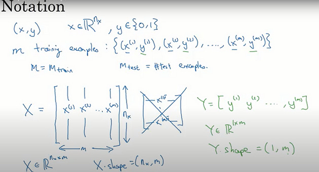
Let’s now lay out some of the notation that we’ll use throughout the rest of this course. A single training example is represented by a pair, (x,y) where x is an x-dimensional feature vector and y, the label, is either 0 or 1. Your training sets will comprise lower-case m training examples. And so your training sets will be written (x1, y1) which is the input and output for your first training example (x(2), y(2)) for the second training example up to (xm, ym) which is your last training example. And then that altogether is your entire training set. So I’m going to use lowercase m to denote the number of training samples. And sometimes to emphasize that this is the number of train examples, I might write this as M = M train. And when we talk about a test set, we might sometimes use m subscript test to denote the number of test examples. So that’s the number of test examples. Finally, to output all of the training examples into a more compact notation, we’re going to define a matrix, capital X. As defined by taking you training set inputs x1, x2 and so on and stacking them in columns. So we take X1 and put that as a first column of this matrix, X2, put that as a second column and so on down to Xm, then this is the matrix capital X. So this matrix X will have M columns,
where M is the number of train examples and the number of railroads, or the height of this matrix is NX. Notice that in other causes, you might see the matrix capital X defined by stacking up the train examples in rows like so, X1 transpose down to Xm transpose. It turns out that when you’re implementing neural networks using this convention I have on the left, will make the implementation much easier. So just to recap, x is a nx by m dimensional matrix, and when you implement this in Python, you see that x.shape, that’s the python command for finding the shape of the matrix, that this an nx, m. That just means it is an nx by m dimensional matrix. So that’s how you group the training examples, input x into matrix. How about the output labels Y? It turns out that to make your implementation of a neural network easier, it would be convenient to also stack Y In columns. So we’re going to define capital Y to be equal to Y 1, Y 2, up to Y m like so. So Y here will be a 1 by m dimensional matrix. And again, to use the notation without the shape of Y will be 1, m. Which just means this is a 1 by m matrix. And as you implement your neural network later in this course you’ll find that a useful convention would be to take the data associated with different training examples, and by data I mean either x or y, or other quantities you see later. But to take the stuff or the data associated with different training examples and to stack them in different columns, like we’ve done here for both x and y. So, that’s a notation we’ll use for a logistic regression and for neural networks networks later in this course. If you ever forget what a piece of notation means, like what is M or what is N or what is something else, we’ve also posted on the course website a notation guide that you can use to quickly look up what any particular piece of notation means. So with that, let’s go on to the next video where we’ll start to fetch out logistic regression using this notation.
Please Follow and 👏 Clap for the story courses teach to see latest updates on this story
🚀 Elevate Your Data Skills with Coursesteach! 🚀
Ready to dive into Python, Machine Learning, Data Science, Statistics, Linear Algebra, Computer Vision, and Research? Coursesteach has you covered!
🔍 Python, 🤖 ML, 📊 Stats, ➕ Linear Algebra, 👁️🗨️ Computer Vision, 🔬 Research — all in one place!
Join the full course for More Learning!🌟

Neural Networks and Deep Learning course
Improving Deep Neural Network course
Stay tuned for our upcoming articles because we reach end to end ,where we will explore specific topics related to Deep Learning in more detail!
We offer following serveries:
We offer the following options:
Enroll in my Deep Learning course: You can sign up for the course at this link. The course is designed in a blog-style format and progresses from basic to advanced levels.
Access free resources: I will provide you with learning materials, and you can begin studying independently. You are also welcome to contribute to our community — this option is completely free.
Online tutoring: If you’d prefer personalized guidance, I offer online tutoring sessions, covering everything from basic to advanced topics.
Contribution: We would love your help in making coursesteach community even better! If you want to contribute in some courses , or if you have any suggestions for improvement in any coursesteach content, feel free to contact and follow.
Together, let’s make this the best AI learning Community! 🚀